Weighted mean depth is a commonly used metric to describe zooplankton populations and vertical distributions. Zooplankton populations can often be found in bimodal patterns throughout the water column, with a subsurface peak and a deeper mesopelagic peak see here. The WMD of a distribution effectively provides a center of mass for the zooplankton in the water column. However, interpreting the WMD often requires context as the depth itself may not be informative. WMD can be particularly useful for DVM studies, as it can show the differences in daytime and nighttime distributions Ohman & Romagnan 2016. Additionally, by calculating the average WMD across multiple samples, the variability (or standard deviation) in WMD can be informative to the overall spread of the zooplankton distribution throughout the water column.
In this study, because profiles extend to different depths and sampling effort (volume) is inconsistent between profiles directly calculating the average WMD is not feasible. However, understanding variation around the WMD is necessary to interpret the vertical structure and strength of DVM. Here, we took a depth-bin constrained bootstrap approach to define WMD with a confidence interval. To do this, the concentration of each group, was calculated in 20m depth bin for each profile. Then all profiles from the same time of day were ‘pooled’. This provides a distribution of concentrations in each depth bin. Traditional bootstrapping randomly samples with replacement from all observations. With vertically structured data however, full random sampling would bias estimates towards the surface, where there were more profiles. To avoid this, samples were “bin-constrained” such that for each iteration, a random observation was sampled within each depth bin, then replaced for the next iteration. A maximum depth was set to 600m, as it is unlikely that copepods are migrated beyond this depth (See figure 3). This approach then effectively created a random profile by resampling a concentration, \(conc^*\), from each depth bin, \(d\). This profile then was used to calculate a bootstrapped weighted mean depth, \(WMD^*\). This was done for each morphological group \(g\), at each time of day \(t\) (\(\ref{Equation 1}\)).
The distribution of \(WMD^*_{g,t}\) then was used to calculate a bootstrapped mean and 95% confidence interval. Then, the confidence intervals could be compared between times of day and morphological groups to assess the strength of DVM. This approach was used to investigate the DVM hypotheses related to size and transparency. Using PC1 to assess size, the WMD was compared between the three PC1-groups by percentile level. Then to assess the effect of transparency, while accounting for size, the WMD was compared between PC2-groups for each PC1-grouping.
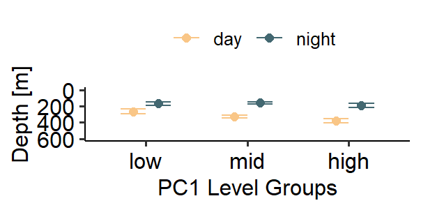
From the visual detection hypothesis, it is predicted that larger and darker copepods will have a larger signal of DVM. A larger signal of DVM would be evident by a clearly deeper (non-overlapping 95% CI) daytime WMD.
Key Figures and Takeaways
For the size assessment, there was a clear signal of DVM across all groups. All the daytime confidence intervals were deeper and non-overlapping with the nighttime intervals. However, the depth of the daytime WMD was different across PC1-groups. The low group had the shallowest WMD (95% CI: [235.2,296.0m]), followed by the middle group (95% CI: [309.0,347.1m]), then the high group (95% CI: [352.3,405.0m]). This pattern provides strong support for the size-dependent DVM hypothesis. The larger a copepod is, the deeper it must migrate during the daytime to avoid visual detection.
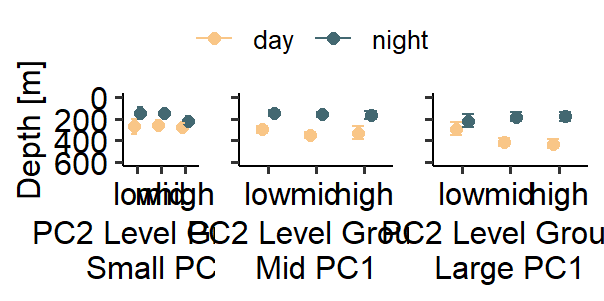
For the influence of transparency, the effect is only clear amongst large (high-PC1 group). For the low-PC1 and mid-PC1 groups, the daytime WMD 95% CI’s are overlapping for all levels of PC2-groups. However, within the larger copepods (high PC1-group), there was a clear signal of weaker DVM by lighter (low PC2-group) copepods. The mid-PC2 and high-PC2 groups had deeper, yet overlapping, daytime 95%CIs. This suggests that some larger copepods can escape the DVM burden through maintaining transparency.
---title: Weighted Mean Depth of Morphological Groups---## MethodologyWeighted mean depth is a commonly used metric to describe zooplankton populations and vertical distributions. Zooplankton populations can often be found in bimodal patterns throughout the water column, with a subsurface peak and a deeper mesopelagic peak [see here](./main_03_Vert-Distrib.html). The WMD of a distribution effectively provides a center of mass for the zooplankton in the water column. However, interpreting the WMD often requires context as the depth itself may not be informative. WMD can be particularly useful for DVM studies, as it can show the differences in daytime and nighttime distributions [Ohman & Romagnan 2016](https://onlinelibrary.wiley.com/doi/abs/10.1002/lno.10251). Additionally, by calculating the average WMD across multiple samples, the variability (or standard deviation) in WMD can be informative to the overall spread of the zooplankton distribution throughout the water column.\n\nIn this study, because profiles extend to different depths and sampling effort (volume) is inconsistent between profiles directly calculating the average WMD is not feasible. However, understanding variation around the WMD is necessary to interpret the vertical structure and strength of DVM. Here, we took a depth-bin constrained bootstrap approach to define WMD with a confidence interval. To do this, the concentration of each group, was calculated in 20m depth bin for each profile. Then all profiles from the same time of day were 'pooled'. This provides a distribution of concentrations in each depth bin. Traditional bootstrapping randomly samples with replacement from all observations. With vertically structured data however, full random sampling would bias estimates towards the surface, where there were more profiles. To avoid this, samples were "bin-constrained" such that for each iteration, a random observation was sampled within each depth bin, then replaced for the next iteration. A maximum depth was set to 600m, as it is unlikely that copepods are migrated beyond this depth (See figure 3). This approach then effectively created a random profile by resampling a concentration, $conc^*$, from each depth bin, $d$. This profile then was used to calculate a bootstrapped weighted mean depth, $WMD^*$. This was done for each morphological group $g$, at each time of day $t$ (\ref{Equation 1}).\begin{align} $WMD^*_{g,t} = \sum_{i}^{N = 60}{\frac{d_i(conc^*_{i,g,t})}{\sum_i^{N = 60}{conc^*_{i,g,t}}}}$ \label{Equation 1}\end{align}The distribution of $WMD^*_{g,t}$ then was used to calculate a bootstrapped mean and 95% confidence interval. Then, the confidence intervals could be compared between times of day and morphological groups to assess the strength of DVM. This approach was used to investigate the DVM hypotheses related to size and transparency. Using PC1 to assess size, the WMD was compared between the three PC1-groups by percentile level. Then to assess the effect of transparency, while accounting for size, the WMD was compared between PC2-groups for each PC1-grouping.From the visual detection hypothesis, it is predicted that larger and darker copepods will have a larger signal of DVM. A larger signal of DVM would be evident by a clearly deeper (non-overlapping 95% CI) daytime WMD.## Key Figures and TakeawaysFor the size assessment, there was a clear signal of DVM across all groups. All the daytime confidence intervals were deeper and non-overlapping with the nighttime intervals. However, the depth of the daytime WMD was different across PC1-groups. The low group had the shallowest WMD (95% CI: [235.2,296.0m]), followed by the middle group (95% CI: [309.0,347.1m]), then the high group (95% CI: [352.3,405.0m]). This pattern provides strong support for the size-dependent DVM hypothesis. The larger a copepod is, the deeper it must migrate during the daytime to avoid visual detection. For the influence of transparency, the effect is only clear amongst large (high-PC1 group). For the low-PC1 and mid-PC1 groups, the daytime WMD 95% CI's are overlapping for all levels of PC2-groups. However, within the larger copepods (high PC1-group), there was a clear signal of weaker DVM by lighter (low PC2-group) copepods. The mid-PC2 and high-PC2 groups had deeper, yet overlapping, daytime 95%CIs. This suggests that some larger copepods can escape the DVM burden through maintaining transparency.\n\n```{r, fig.width=3.15, fig.height=1.57}rm(list =ls())library(ggplot2)library(ggpubr)source('../r/tools.R')boot_wmd <-readRDS('../data/03b_alt-mg-wmd-bins.rds')# |- Summarize DF -----------------------summarize_wmd <-function(wmd_group) { day_summary <- wmd_group$day |>lapply(quantile, probs =c(0.025,0.5,.975)) night_summary <- wmd_group$night |>lapply(quantile, probs =c(0.025,0.5,0.975)) wmd_df <-data.frame(group =rep(c('low','mid','high'), each =2),tod =rep(c('day','night'), times =3),lbound =rep(NA,6),mean =rep(NA,6),hbound =rep(NA,6))for(group inc('low','mid','high')) { wmd_df[['lbound']][which(wmd_df[['tod']] =='day'& wmd_df[['group']] == group)] <- day_summary[[group]][['2.5%']] wmd_df[['mean']][which(wmd_df[['tod']] =='day'& wmd_df[['group']] == group)] <-mean(wmd_group$day[[group]]) wmd_df[['hbound']][which(wmd_df[['tod']] =='day'& wmd_df[['group']] == group)] <- day_summary[[group]][['97.5%']] wmd_df[['lbound']][which(wmd_df[['tod']] =='night'& wmd_df[['group']] == group)] <- night_summary[[group]][['2.5%']] wmd_df[['mean']][which(wmd_df[['tod']] =='night'& wmd_df[['group']] == group)] <-mean(wmd_group$night[[group]]) wmd_df[['hbound']][which(wmd_df[['tod']] =='night'& wmd_df[['group']] == group)] <- night_summary[[group]][['97.5%']] } wmd_df$group <-factor(wmd_df$group, levels =c('low','mid','high'))return(wmd_df)}pc1_wmd_df <- boot_wmd$pc1 |>summarize_wmd()pc1_plot <-ggplot(pc1_wmd_df) +geom_point(aes(x = group,y = mean,color = tod),position =position_dodge(width = .5),size =2) +geom_errorbar(aes(x = group,ymin = lbound,ymax = hbound,color = tod),width = .5,position =position_dodge(width = .5),size = .5) +scale_color_manual(values =c(dn_cols['day'],dn_cols['night'])) +scale_y_reverse(limits =c(600,0)) +labs(y ='Depth [m]', x ='PC1 Level Groups', col ="")+theme_pubr()pc1_plot# # ggsave('../media/raw_04_figure.pdf', pc1_plot,# width = 80, height = 80, units = 'mm',# dpi = 600)knitr::kable(pc1_wmd_df)```Observe for PC2 breaks by PC1 group```{r, fig.width=3.15, fig.height=1.57}small_pc2 <- boot_wmd$pc2_sm |>summarize_wmd()mid_pc2 <- boot_wmd$pc2_mid |>summarize_wmd()lg_pc2 <- boot_wmd$pc2_lg |>summarize_wmd()pc2_plotter <-function(wmd, pc1_group){ggplot(wmd) +geom_point(aes(x = group,y = mean,color = tod),position =position_dodge(width = .5),size =2) +geom_errorbar(aes(x = group,ymin = lbound,ymax = hbound,color = tod),width = .5,position =position_dodge(width = .5),size = .5) +scale_color_manual(values =c(dn_cols['day'],dn_cols['night'])) +scale_y_reverse(limits =c(600,0)) +labs(y ='Depth [m]', x =paste0('PC2 Level Groups','\n',pc1_group), col ="")+theme_pubr()}sm_plot <-pc2_plotter(small_pc2, 'Small PC1')mid_plot <-pc2_plotter(mid_pc2, 'Mid PC1')lg_plot <-pc2_plotter(lg_pc2, 'Large PC1')pc2_plot <-ggarrange(sm_plot, mid_plot +theme(axis.title.y =element_blank(),axis.text.y =element_blank()), lg_plot +theme(axis.title.y =element_blank(),axis.text.y =element_blank()),ncol =3, common.legend = T, widths =c(1,.9,.9))pc2_plot# ggarrange(pc1_plot,# pc2_plot,# nrow = 2)ggsave('../media/raw_05_figure.pdf', pc2_plot,width =180, height =80, units ='mm',dpi =600)``````{r}DT::datatable(small_pc2, caption ='Small PC1 - PC2 Groups')DT::datatable(mid_pc2, caption ='Mid PC1 - PC2 Groups')DT::datatable(lg_pc2, caption ='Large PC1 - PC2 Groups')```