Code
rm(list = ls())
library(DT)
library(EcotaxaTools)
library(ggplot2)
library(ggpubr)


pca_results <- readRDS('../data/02_cope-pca-res.rds')Additional Information related to the PCA used in this analysis are visible here. View the main conclusions from the analysis here.
rm(list = ls())
library(DT)
library(EcotaxaTools)
library(ggplot2)
library(ggpubr)
pca_results <- readRDS('../data/02_cope-pca-res.rds')# |- make a circle for plotting variable contributions -------------------
curl <- seq(-pi,pi, length = 50)
circ <- data.frame(x = sin(curl), y = cos(curl))
# |- Extract variable contributions ----------------------------
pc_df <- data.frame(
pc1 = pca_results$var$coord[,1],
pc2 = pca_results$var$coord[,2],
pc3 = pca_results$var$coord[,3],
pc4 = pca_results$var$coord[,4],
vars = row.names(pca_results$var$coord)
)
pc1_pc2 <- ggplot() +
geom_path(data = circ,aes(x,y), lty = 2, color = "grey", alpha = 0.7) +
geom_text(data = pc_df, aes(x = pc1, y = pc2, label = vars),
position = position_jitter()) +
geom_segment(data = pc_df,
aes(x = 0, y = 0, xend = pc1*0.9, yend = pc2*0.9),
arrow = arrow(length = unit(1/2, 'picas')), color = "grey30") +
labs(x = 'PC1 - 34.23%',y = 'PC2 - 27.24%')+
theme_pubclean()+
theme(panel.border = element_rect(fill = 'transparent'))
pc3_pc4 <- ggplot() +
geom_path(data = circ,aes(x,y), lty = 2, color = "grey", alpha = 0.7) +
geom_text(data = pc_df, aes(x = pc3, y = pc4, label = vars),
position = position_jitter()) +
geom_segment(data = pc_df,
aes(x = 0, y = 0, xend = pc3*0.9, yend = pc4*0.9),
arrow = arrow(length = unit(1/2, 'picas')), color = "grey30") +
labs(x = 'PC3 - 17.05%',y = 'PC4 - 09.38%')+
theme_pubclean()+
theme(panel.border = element_rect(fill = 'transparent'))
ggarrange(pc1_pc2, pc3_pc4)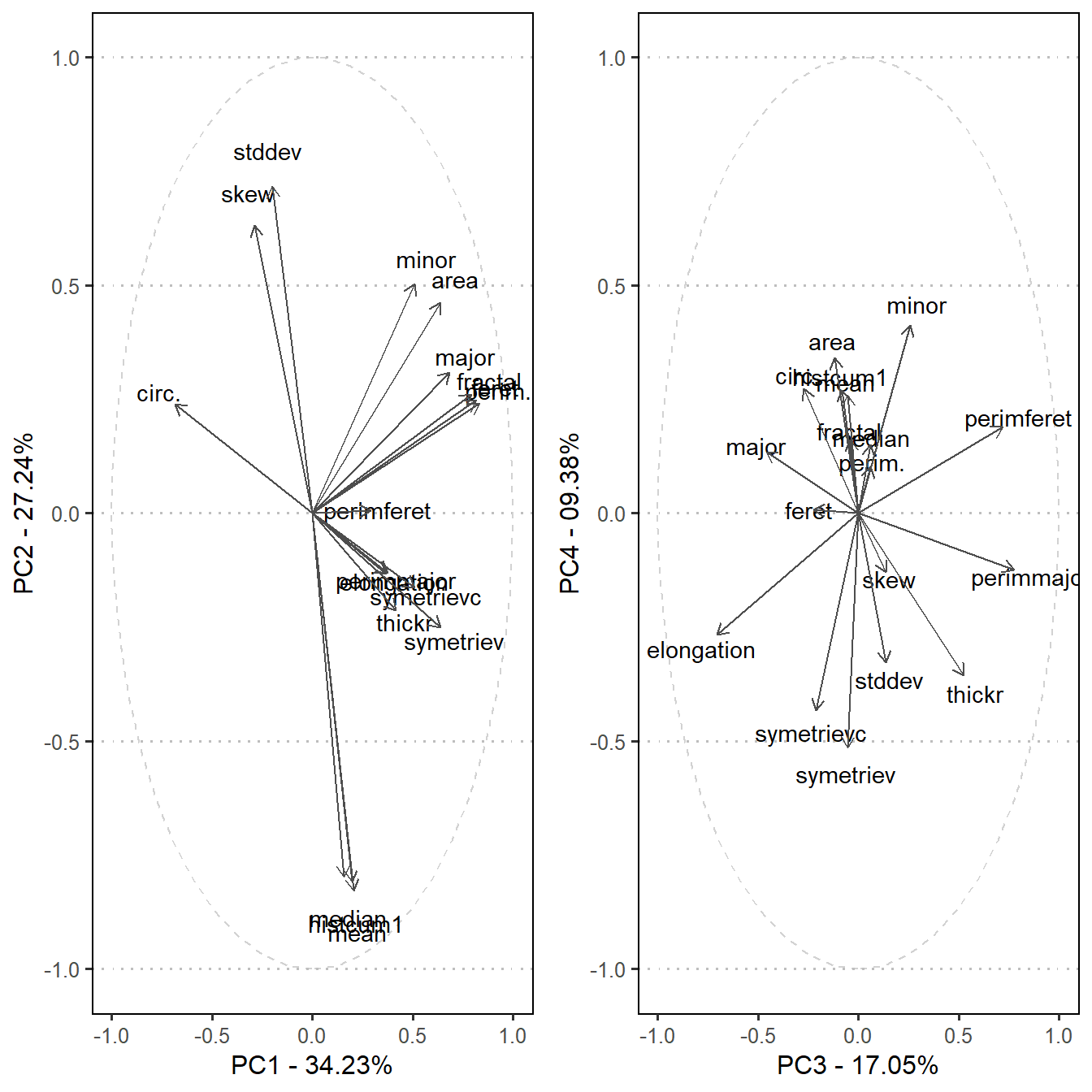
Specific loading scores are available for each of the four dimensions:
datatable(pca_results$var$coord[,c(1:4)])