To understand the vertical distribution of the different morphological groups, the concentration of each group was calculated in a 20m-bin. Groups were identified based on their PC1 and PC2 percentile groups. The binned concentrations were averaged across all profiles in the study (following the average-cast method described in Barth & Stone 2022. Using the average-cast approach is beneficial as it allows for data to be included from casts with different max descents, so long as an entire 20m depth bin was sampled, it is included. Averages were calculated separately for daytime and nighttime casts.
Figures & Take-aways:
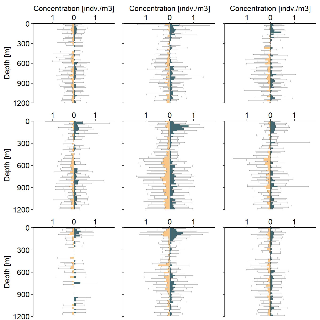
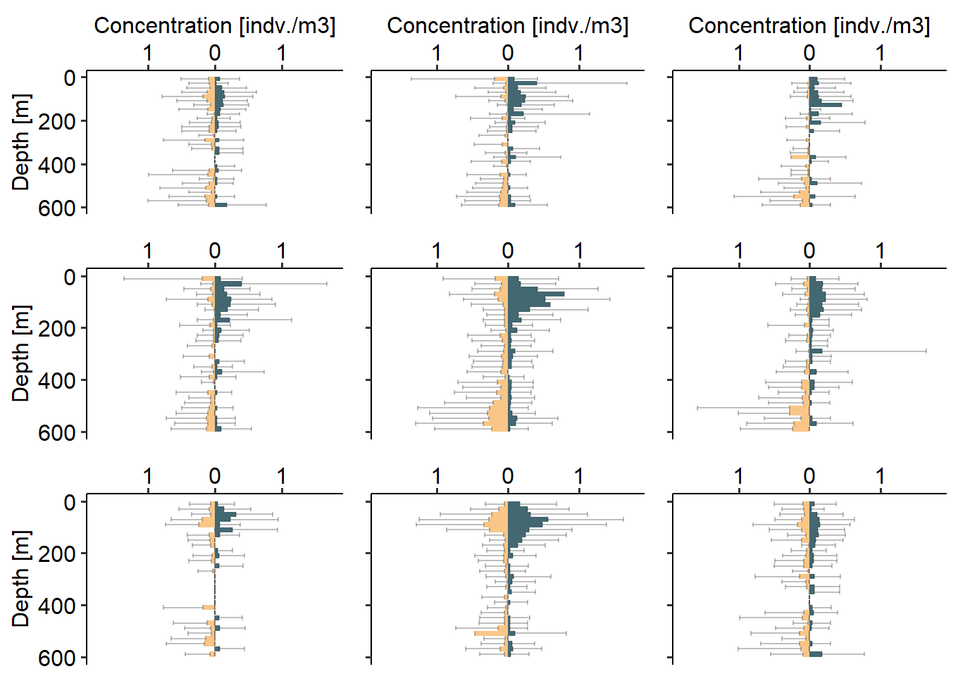
There was an evident day/night difference in the average vertical structure across all morphological groups. This pattern is primarily in the upper 600m. While there were copepods observed throughout the mesopelagic, there was not a noticable difference between the day and nighttime average concentrations. Additionally, the variation between casts was extremely large, as seen with the standard deviation of different profiles. Often the standard deviation of depth-bin abundance is much larger than the average abundance. This is in part driven by high variability between cruises which occurred in different seasonsgetting averaged together. However, there is also large variability between individual casts, which can be driven by the small sampling volume of the UVP as described by Barth & Stone 2022.
Code
##### Get project-wide night-day differences ###########rm(list =ls())library(EcotaxaTools)library(ggplot2)library(ggpubr)source('../R/tools.R')uvp_data <-readRDS('../data/01_uvp-trim-final_large.rds') |>trim_to_cope()pc2_bin_sm <-readRDS('../data/03b_pc2-sm-bins.rds')pc2_bin_mid <-readRDS('../data/03b_pc2-bins.rds')pc2_bin_lg <-readRDS('../data/03b_pc2-lg-bins.rds')# |- Reformat PC group names --------------------# group names will be pc1_pc2: e.g. low-low, low-mid, etc# assign pc1-class to eachgroup_renamer <-function(x, pc1_group) { x$group <-paste0(pc1_group, '_', x$group)return(x)}pc2_bin_lg <- pc2_bin_lg |>lapply(group_renamer, 'high') |>assign_etx_class('zoo_conc_list')pc2_bin_mid <- pc2_bin_mid |>lapply(group_renamer, 'mid')|>assign_etx_class('zoo_conc_list')pc2_bin_sm <- pc2_bin_sm |>lapply(group_renamer, 'low')|>assign_etx_class('zoo_conc_list')# |- Merger into a single conc list ---------------bin_merger <-function(profileid) { lg_df <- pc2_bin_lg[[profileid]] mid_df <- pc2_bin_mid[[profileid]] sm_df <- pc2_bin_sm[[profileid]]return(do.call(rbind, list(lg_df, mid_df, sm_df)))}all_casts <- uvp_data$meta$profileid |>lapply(bin_merger)names(all_casts) <- uvp_data$meta$profileidcast_times <-list(day = uvp_data$meta$profileid[which(uvp_data$meta$tod =='day')],night = uvp_data$meta$profileid[which(uvp_data$meta$tod =='night')])avg_cope <- all_casts |>average_casts(cast_times) |>lapply(bin_format)
---title: Vertical Distribution of Morphotypes---## Methodology:To understand the vertical distribution of the different morphological groups, the concentration of each group was calculated in a 20m-bin. Groups were identified based on their PC1 and PC2 percentile groups. The binned concentrations were averaged across all profiles in the study (following the average-cast method described in [Barth & Stone 2022](https://thealexbarth.github.io/Oligotrophic_in-situ_net_comparison/main_analysis_03.html). Using the average-cast approach is beneficial as it allows for data to be included from casts with different max descents, so long as an entire 20m depth bin was sampled, it is included. Averages were calculated separately for daytime and nighttime casts.## Figures & Take-aways:There was an evident day/night difference in the average vertical structure across all morphological groups. This pattern is primarily in the upper 600m. While there were copepods observed throughout the mesopelagic, there was not a noticable difference between the day and nighttime average concentrations. Additionally, the variation between casts was extremely large, as seen with the standard deviation of different profiles. Often the standard deviation of depth-bin abundance is much larger than the average abundance. This is in part driven by high variability between cruises which occurred in different seasonsgetting averaged together. However, there is also large variability between individual casts, which can be driven by the small sampling volume of the UVP as described by [Barth & Stone 2022](https://www.frontiersin.org/articles/10.3389/fmars.2022.898057/full).```{r}##### Get project-wide night-day differences ###########rm(list =ls())library(EcotaxaTools)library(ggplot2)library(ggpubr)source('../R/tools.R')uvp_data <-readRDS('../data/01_uvp-trim-final_large.rds') |>trim_to_cope()pc2_bin_sm <-readRDS('../data/03b_pc2-sm-bins.rds')pc2_bin_mid <-readRDS('../data/03b_pc2-bins.rds')pc2_bin_lg <-readRDS('../data/03b_pc2-lg-bins.rds')# |- Reformat PC group names --------------------# group names will be pc1_pc2: e.g. low-low, low-mid, etc# assign pc1-class to eachgroup_renamer <-function(x, pc1_group) { x$group <-paste0(pc1_group, '_', x$group)return(x)}pc2_bin_lg <- pc2_bin_lg |>lapply(group_renamer, 'high') |>assign_etx_class('zoo_conc_list')pc2_bin_mid <- pc2_bin_mid |>lapply(group_renamer, 'mid')|>assign_etx_class('zoo_conc_list')pc2_bin_sm <- pc2_bin_sm |>lapply(group_renamer, 'low')|>assign_etx_class('zoo_conc_list')# |- Merger into a single conc list ---------------bin_merger <-function(profileid) { lg_df <- pc2_bin_lg[[profileid]] mid_df <- pc2_bin_mid[[profileid]] sm_df <- pc2_bin_sm[[profileid]]return(do.call(rbind, list(lg_df, mid_df, sm_df)))}all_casts <- uvp_data$meta$profileid |>lapply(bin_merger)names(all_casts) <- uvp_data$meta$profileidcast_times <-list(day = uvp_data$meta$profileid[which(uvp_data$meta$tod =='day')],night = uvp_data$meta$profileid[which(uvp_data$meta$tod =='night')])avg_cope <- all_casts |>average_casts(cast_times) |>lapply(bin_format)``````{r, out.width='100%', fig.width=7.087, fig.height=7.087}#| column: page-outset#### Create group profiles ######## |- Concentration Profile --------------------------------------------group_profile <-function(g) { ret_plot <-ggplot()+geom_rect(data = avg_cope$day[avg_cope$day$group == g,],aes(xmin = min_d, xmax = max_d,ymin =0, ymax =-mean),fill = dn_cols['day']) +geom_errorbar(data = avg_cope$day[avg_cope$day$group == g,],aes(x = mp, ymin =-mean, ymax =-(mean+sd)),alpha = .25) +geom_rect(data = avg_cope$night[avg_cope$night$group == g,],aes(xmin = min_d, xmax = max_d,ymin =0, ymax = mean),fill = dn_cols['night']) +geom_errorbar(data = avg_cope$night[avg_cope$night$group == g,],aes(x = mp, ymin = mean, ymax = (mean+sd)),alpha = .25)+labs(x ='Depth [m]', y ='Concentration [indv./m3]')+coord_flip()+scale_x_reverse(expand =c(0,0))+scale_y_continuous(position ='right',labels = abs,limits =c(-1.75,1.75)) +theme_pubr()return(ret_plot)}group_cats <-c('low_high','mid_high','high_high','low_mid','mid_mid','high_mid','low_low','mid_low','high_low')plot_list <-list()for(g in group_cats) { plot_list[[g]] <-group_profile(g)}y_axis_clear <-theme(axis.text.y =element_blank(),axis.title.y =element_blank())x_axis_clear <-theme(axis.title.x =element_blank())both_axis_clear <- y_axis_clear + x_axis_clearggarrange(plot_list$low_high, #TL plot_list$mid_high + y_axis_clear, #TM plot_list$high_high + y_axis_clear, #TR plot_list$mid_high + x_axis_clear, #ML plot_list$mid_mid + both_axis_clear, #MM plot_list$high_mid + both_axis_clear, #MR plot_list$low_low + x_axis_clear, #BL plot_list$low_mid + both_axis_clear, #BM plot_list$low_high + both_axis_clear, #BRnrow =3, ncol =3,widths =c(1,.85,.85,1,.85,.85,1,.85,.85))```We can zoom in on the upper 600m to get a better picture of the changes in the upper layers.```{r, out.width='100%', fig.width = 7.087, fig.width=7.087}#| column: screen-insetshort_plot <-ggarrange(plot_list$low_high +xlim(600,0), #TL plot_list$mid_high + y_axis_clear +xlim(600,0), #TM plot_list$high_high + y_axis_clear +xlim(600,0), #TR plot_list$mid_high + x_axis_clear +xlim(600,0), #ML plot_list$mid_mid + both_axis_clear +xlim(600,0), #MM plot_list$high_mid + both_axis_clear +xlim(600,0), #MR plot_list$low_low + x_axis_clear +xlim(600,0), #BL plot_list$low_mid + both_axis_clear +xlim(600,0), #BM plot_list$low_high + both_axis_clear +xlim(600,0), #BRnrow =3, ncol =3,widths =c(1,.85,.85,1,.85,.85,1,.85,.85))short_plot# ggsave('../media/raw_03_figure.pdf',short_plot,# height = 170, width = 170, units = 'mm', dpi = 600)```