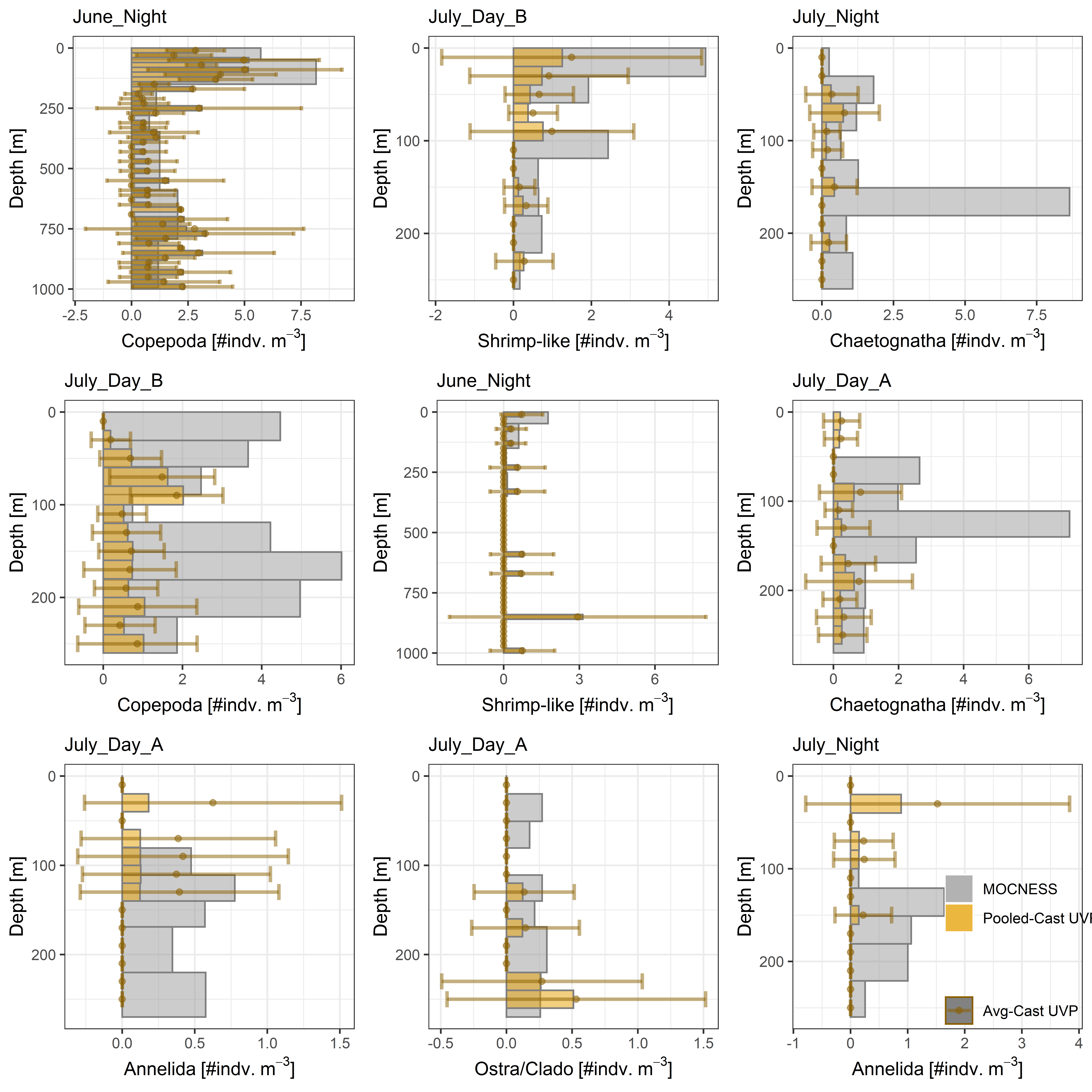
Select Density Profiles

Density profiles of comparable taxa are shown when measured by the MOCNESS/ZOOSCAN and the UVP. All MOCNESS data are for plankton larger than 0.934mm. MOCNESS depth bins were determined by net-deployments. UVP depth bins are shown in 20m-bins. The UVP bin size is an import consideration when calculating UVP abundance profiles. Density estimates from the UVP were calculated two ways. In one method (pooled-cast), similar UVP casts are pooled then the density of organisms in a depth bin were calculated. \[\frac{\sum_{i}^{N}individuals_{i}}{\sum_{i}^{N}volume sampled_{i}}\] The other method (averaged-cast), density is calculated in individual uvp casts, then averaged between all similar casts: \[\frac{\sum_{i=1}^{N} \frac{individuals_{i}}{volume sampled_{i}}}{N}\] For all i casts, with a total of N casts.

Code

rm(list = ls())
library(cowplot)
library(ggplot2)
plot_list <- readRDS('../Output/main_fig_03_profile-density-comparison.rds')

Code

grid_theme <- theme(legend.position = 'none')
plot_grid(plot_list$June_Night_Copepoda + grid_theme,
          plot_list$`July_Day_B_Shrimp-like` + grid_theme,
          plot_list$July_Night_Chaetognatha+ grid_theme,
          plot_list$July_Day_B_Copepoda + grid_theme,
          plot_list$`June_Night_Shrimp-like` + grid_theme,
          plot_list$July_Day_A_Chaetognatha + grid_theme,
          plot_list$July_Day_A_Annelida + grid_theme,
          plot_list$`July_Day_A_Ostra/Clado`+ grid_theme,
          plot_list$July_Night_Annelida + theme(legend.position = c(.80,.35)),
          ncol = 3)

Select taxa depth profiles. Pooled-UVP cast estimates are shown as barplots. Averaged-UVP casts estimates are shown by points with standard deviation shown.

Select Profiles are shown to highlight cases where: the vertical patterns measured by the MOCNESS are matched by the UVP (top row), the vertical patterns measured by the MOCNESS are not well matched by the UVP (mid row), and cases where the UVP captured organisms in depth regions where the MOCNESS did not (bottom row). All casts can be seen in Supplemental Figure 6.

These patterns show that the UVP and MOCNESS are inconsistent in their measurements of zooplankton communities. The pooled-cast UVP estimation method consistently underestimates zooplantkon densities for all taxa. However, the average-cast UVP estimation method is at times larger or lower than MOCNESS estimates in similar depth regions. The average-cast method does however allow for ability to measure variance between similar casts. For sparser organisms, this variance is is likely driven by the low sampling volume of the UVP. However, for organisms which occur in larger numbers (Copepoda & Shrimp-like crustaceans), patchiness of the plankton likely drive variation between casts. Users of the UVP need to consider the

---
title: "Select Density Profiles"
---

Density profiles of comparable taxa are shown when measured by the MOCNESS/ZOOSCAN and the UVP. All MOCNESS data are for plankton larger than 0.934mm. MOCNESS depth bins were determined by net-deployments. UVP depth bins are shown in 20m-bins. The UVP bin size is an [import consideration](./supp_analysis_04.html) when calculating UVP abundance profiles. Density estimates from the UVP were calculated two ways. In one method (pooled-cast), similar UVP casts are pooled then the density of organisms in a depth bin were calculated. $$\frac{\sum_{i}^{N}individuals_{i}}{\sum_{i}^{N}volume sampled_{i}}$$ The other method (averaged-cast), density is calculated in individual uvp casts, then averaged between all similar casts: $$\frac{\sum_{i=1}^{N} \frac{individuals_{i}}{volume sampled_{i}}}{N}$$ For all i casts, with a total of N casts.



```{r warning=F, message=F}
rm(list = ls())
library(cowplot)
library(ggplot2)
plot_list <- readRDS('../Output/main_fig_03_profile-density-comparison.rds')
```


```{r All-Plots, fig.height=9,fig.width=9,fig.cap='Select taxa depth profiles. Pooled-UVP cast estimates are shown as barplots. Averaged-UVP casts estimates are shown by points with standard deviation shown.', dpi = 500}
#| column: body-outset

grid_theme <- theme(legend.position = 'none')
plot_grid(plot_list$June_Night_Copepoda + grid_theme,
          plot_list$`July_Day_B_Shrimp-like` + grid_theme,
          plot_list$July_Night_Chaetognatha+ grid_theme,
          plot_list$July_Day_B_Copepoda + grid_theme,
          plot_list$`June_Night_Shrimp-like` + grid_theme,
          plot_list$July_Day_A_Chaetognatha + grid_theme,
          plot_list$July_Day_A_Annelida + grid_theme,
          plot_list$`July_Day_A_Ostra/Clado`+ grid_theme,
          plot_list$July_Night_Annelida + theme(legend.position = c(.80,.35)),
          ncol = 3)
```
-------------------------------------------------------------------------------

Select Profiles are shown to highlight cases where: the vertical patterns measured by the MOCNESS are matched by the UVP (top row), the vertical patterns measured by the MOCNESS are not well matched by the UVP (mid row), and cases where the UVP captured organisms in depth regions where the MOCNESS did not (bottom row). All casts can be seen in [Supplemental Figure 6](./supp_analysis_06.html).

------------------------------------------------------------------------------

These patterns show that the UVP and MOCNESS are inconsistent in their measurements of zooplankton communities. The pooled-cast UVP estimation method consistently underestimates zooplantkon densities for all taxa. However, the average-cast UVP estimation method is at times larger or lower than MOCNESS estimates in similar depth regions. The average-cast method does however allow for ability to measure variance between similar casts. For sparser organisms, this variance is is likely driven by the low sampling volume of the UVP. However, for organisms which occur in larger numbers (Copepoda & Shrimp-like crustaceans), patchiness of the plankton likely drive variation between casts. Users of the UVP need to consider the