The MOCNESS and UVP inherently sample different size ranges. The MOCNESS was equipped with 153 micron mesh while the UVP only saves particles above 600 microns. To compare the effectiveness of the two devices, we analyzed MOCNESS images equal to or larger to what we are able to measure with the UVP. This comparison focuses only on taxa which made up a substantial portion of taxa sampled by both instruments. It is important to note that although UVP is set to save particle images above 600 microns, for comparable sized taxa, larger sizes are needed to accurately distinguish plankton from particles. The smallest recorded comparable organism was a 934 micron Shrimp-like crustacean. As such, this was the minimum size for inclusion for any MOCNESS-collected plankton in subsequent analyses. The full MOCNESS size range extends to much smaller organisms
Here we compare All taxa, Annelids, Chaetognaths, Copepods, Shrimp-like Crustaceans, and Ostracod/Cladoceans.
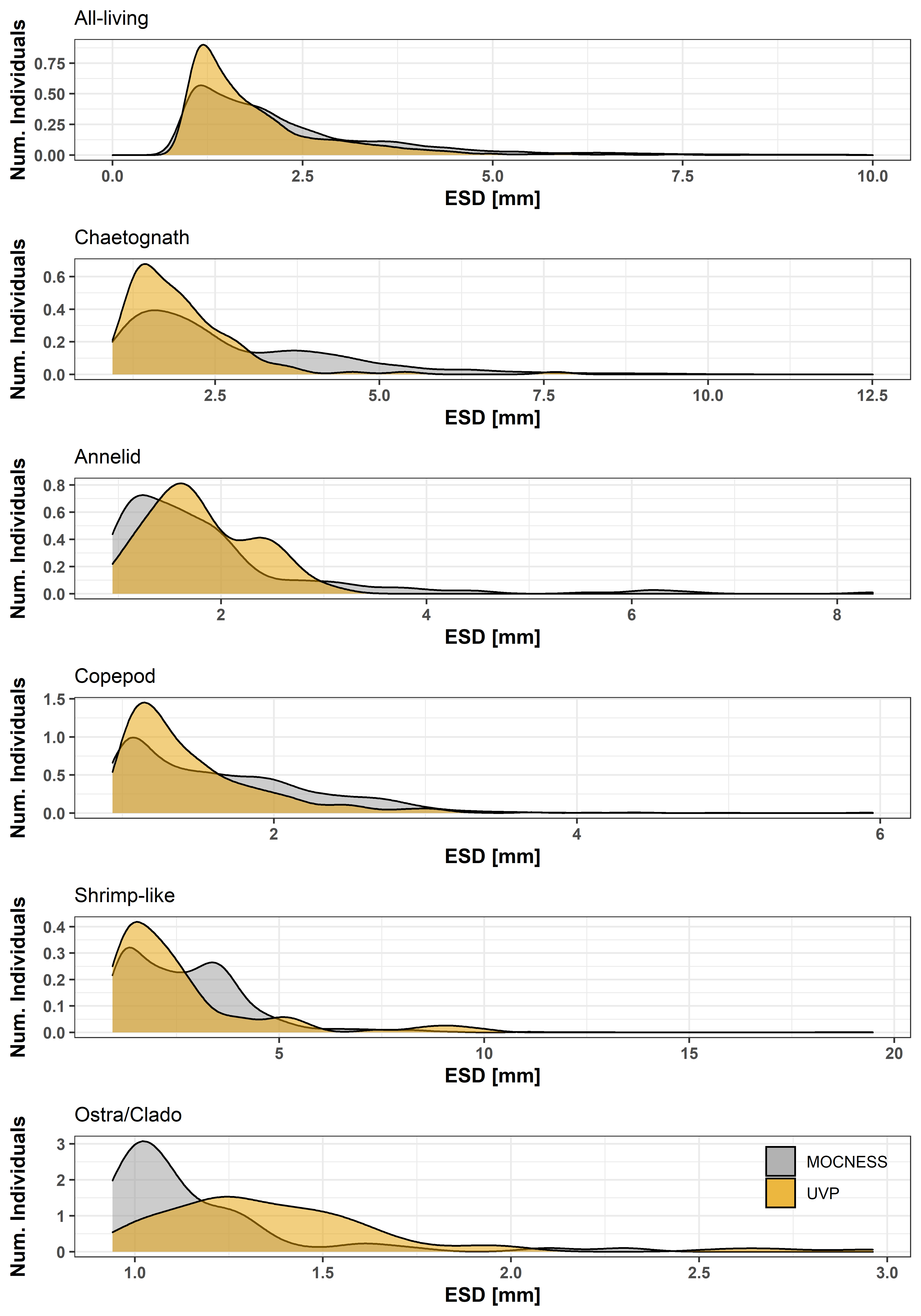
Size distributions for select taxa. MOCNESS individuals below 0.934mm were excluded
Notably, there is a large size overlap for many of the taxa. However, there is a portion of large Copepods, Chaetognaths, and Shrimp-like crustaceans sampled by the MOCNESS which are seemingly undersampled by the UVP. This is possibly due to avoidance of the UVP by these large, mobile organisms. The UVP samples a slightly larger range of annlids. However this observation is likely due to polychaetes getting broken into smaller fragments in the MOCNESS, and thus not representative of their in situ size. Additionally, the UVP samples a larger size range of Ostracods/Cladocerans. However, this may be an artefact of the inability to identify smaller cladocerans in UVP images.
Code
comp_taxo <-c('Chaetognatha', 'Annelida', 'Copepoda', 'Shrimp-like','Ostra/Clado')# Format the data for the tablesummary_df <-function(df, sum_col, sum_by) { rdf <-data.frame(taxa =sort(unique(df[[sum_by]])),min =rep(NA, length(unique(df[[sum_by]]))),median =rep(NA, length(unique(df[[sum_by]]))),mean =rep(NA, length(unique(df[[sum_by]]))),max =rep(NA, length(unique(df[[sum_by]])))) rdf$min <-aggregate(df[[sum_col]], by =list(taxa = df[[sum_by]]),FUN = min)$x rdf$median <-aggregate(df[[sum_col]], by =list(taxa = df[[sum_by]]),FUN = median)$x rdf$mean <-aggregate(df[[sum_col]], by =list(taxa = df[[sum_by]]),FUN = mean)$x rdf$max <-aggregate(df[[sum_col]], by =list(taxa = df[[sum_by]]),FUN = max)$x all_sum <-data.frame(taxa ='All-Living') all_sum$min <-min(df[[sum_col]]) all_sum$median <-median(df[[sum_col]]) all_sum$mean <-mean(df[[sum_col]]) all_sum$max <-max(df[[sum_col]]) rdf <-rbind(all_sum, rdf)return(rdf)}moc_dat <-summary_df(dat_list$moc_trim, 'calc_esd', 'taxo_name')uvp_dat <-summary_df(dat_list$uvp, 'calc_esd', 'name')datatable(moc_dat, class ='hover', caption ='Size summary statistics for MOCNESS-collected plankton above 0.934mm. Units are mm.',rownames = F)
Source Code
---title: Comparison of Size Distributions Sampled by two devices---```{r importing data, warning=FALSE}rm(list =ls())library(ggplot2)library(EcotaxaTools)library(DT)library(cowplot)dat_list <-readRDS('../Output/data_01_size-range-dfs.rds')plot_list <-readRDS('../Output/main_fig_01_matched-size-distribution.rds')load('../Output/data_01_plotting-needs.rda')```The MOCNESS and UVP inherently sample different size ranges. The MOCNESS was equipped with 153 micron mesh while the UVP only saves particles above 600 microns. To compare the effectiveness of the two devices, we analyzed MOCNESS images equal to or larger to what we are able to measure with the UVP. This comparison focuses only on taxa which made up a [substantial](./main_analysis_02.html) portion of taxa sampled by both instruments. It is important to note that although UVP is set to save particle images above 600 microns, for comparable sized taxa, larger sizes are needed to accurately distinguish plankton from particles. The smallest recorded comparable organism was a 934 micron Shrimp-like crustacean. As such, this was the minimum size for inclusion for any MOCNESS-collected plankton in subsequent analyses. The full MOCNESS size range extends to much [smaller organisms](./supp_analysis_05.html)Here we compare All taxa, Annelids, Chaetognaths, Copepods, Shrimp-like Crustaceans, and Ostracod/Cladoceans.```{r Figure 1, fig.height=10, out.width='100%',fig.cap= 'Size distributions for select taxa. MOCNESS individuals below 0.934mm were excluded', dpi= 300, message = F, warning = F}#| column: body-outsetgrid_theme <-theme(legend.position ='none')plot_grid(plot_list[[1]]+grid_theme+labs(subtitle ='All-living'), plot_list[[2]]+grid_theme+labs(subtitle ='Chaetognath'), plot_list[[3]]+grid_theme+labs(subtitle ='Annelid'), plot_list[[4]]+grid_theme+labs(subtitle ='Copepod'), plot_list[[5]]+grid_theme+labs(subtitle ='Shrimp-like'), plot_list[[6]]+labs(subtitle ='Ostra/Clado'),align ='vh',ncol =1)```------------------------------------------------------------------------Notably, there is a large size overlap for many of the taxa. However, there is a portion of large Copepods, Chaetognaths, and Shrimp-like crustaceans sampled by the MOCNESS which are seemingly undersampled by the UVP. This is possibly due to avoidance of the UVP by these large, mobile organisms. The UVP samples a slightly larger range of annlids. However this observation is likely due to polychaetes getting broken into smaller fragments in the MOCNESS, and thus not representative of their *in situ* size. Additionally, the UVP samples a larger size range of Ostracods/Cladocerans. However, this may be an artefact of the inability to identify smaller cladocerans in UVP images.------------------------------------------------------------------------```{r Summary table}#| column: screen-insetcomp_taxo <-c('Chaetognatha', 'Annelida', 'Copepoda', 'Shrimp-like','Ostra/Clado')# Format the data for the tablesummary_df <-function(df, sum_col, sum_by) { rdf <-data.frame(taxa =sort(unique(df[[sum_by]])),min =rep(NA, length(unique(df[[sum_by]]))),median =rep(NA, length(unique(df[[sum_by]]))),mean =rep(NA, length(unique(df[[sum_by]]))),max =rep(NA, length(unique(df[[sum_by]])))) rdf$min <-aggregate(df[[sum_col]], by =list(taxa = df[[sum_by]]),FUN = min)$x rdf$median <-aggregate(df[[sum_col]], by =list(taxa = df[[sum_by]]),FUN = median)$x rdf$mean <-aggregate(df[[sum_col]], by =list(taxa = df[[sum_by]]),FUN = mean)$x rdf$max <-aggregate(df[[sum_col]], by =list(taxa = df[[sum_by]]),FUN = max)$x all_sum <-data.frame(taxa ='All-Living') all_sum$min <-min(df[[sum_col]]) all_sum$median <-median(df[[sum_col]]) all_sum$mean <-mean(df[[sum_col]]) all_sum$max <-max(df[[sum_col]]) rdf <-rbind(all_sum, rdf)return(rdf)}moc_dat <-summary_df(dat_list$moc_trim, 'calc_esd', 'taxo_name')uvp_dat <-summary_df(dat_list$uvp, 'calc_esd', 'name')datatable(moc_dat, class ='hover', caption ='Size summary statistics for MOCNESS-collected plankton above 0.934mm. Units are mm.',rownames = F)``````{r Second table, echo = FALSE}#| column: screen-insetdatatable(uvp_dat, class ='hover', caption ='Size summary statistics for plankton imaged by the UVP',rownames = F)```