Regression of density estimates
To compare similarity of UVP and MOCNESS estimates of taxa abundance, linear regressions were constructed to compare estimates between the devices of similarly sized taxa (above 0.934mm) in matching depth bins.
UVP Estimates were calculated following both a pooled-cast approach and an average-cast approach. See methods for calculation here.
Below are plotted results. Grey lines indicate the 1:1 line (if estimates were equal between the devices). Black lines indicate the line of best fit.
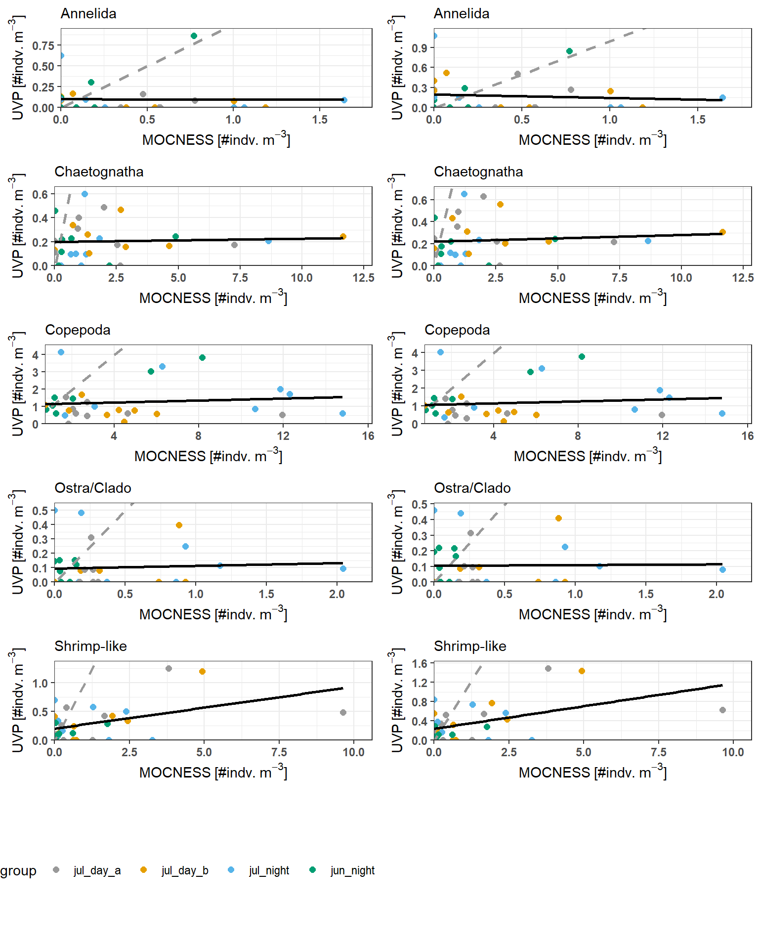
Across all taxa, there are no clear relationships between MOCNESS and UVP estimates in similar depth bins. There is a significant relationship between density estimates for Shrimp-like crustaceans (with both UVP methods), however this is likely driven by the high-influence outliers. It is also clear from the plot that there are high residual heteroskedasticty in all regressions.
Regression summaries can be found below: ::: {.cell}
Code
get_reg_sum <- function(reg) {
  reg_summary <- summary(reg)
  rvect <- reg_summary$coefficients[2,-3]
  rvect[4] <- reg_summary$r.squared
  names(rvect) <- c('Slope_Estimate','Std.Error','p-value','r.squared')
  return(rvect)
}
pool_sum <- lapply(reg_dat$pooled, get_reg_sum) |> list_to_tib('Taxa')
avg_sum <- lapply(reg_dat$avged, get_reg_sum) |> list_to_tib('Taxa')
#| Column: body-outset
DT::datatable(pool_sum, class = 'hover', caption = 'Pooled-cast method UVP vs MOCNESS regression output')
Code
#| Column: body-outset
DT::datatable(avg_sum, class = 'hover', caption = 'Average-cast method UVP vs MOCNESS regression output')
:::