Code
rm(list = ls())
library(cowplot)
library(ggplot2)
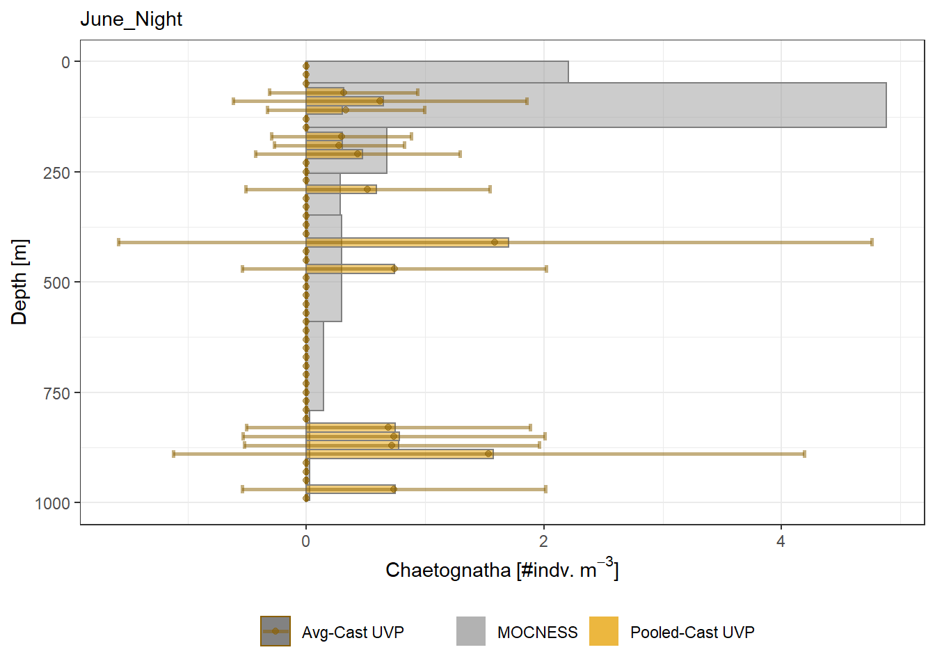
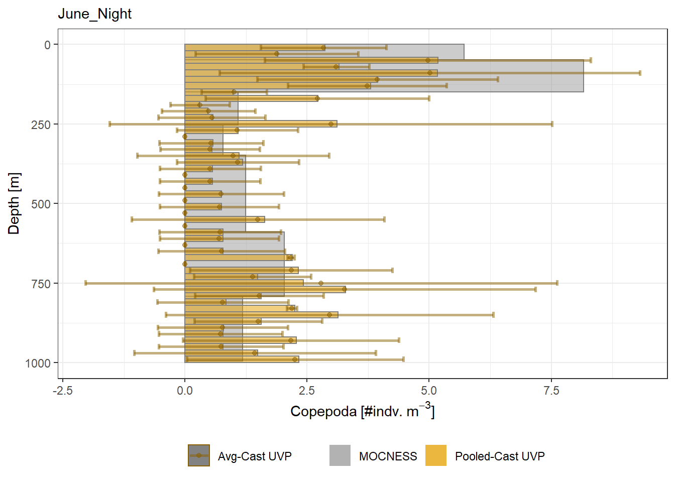
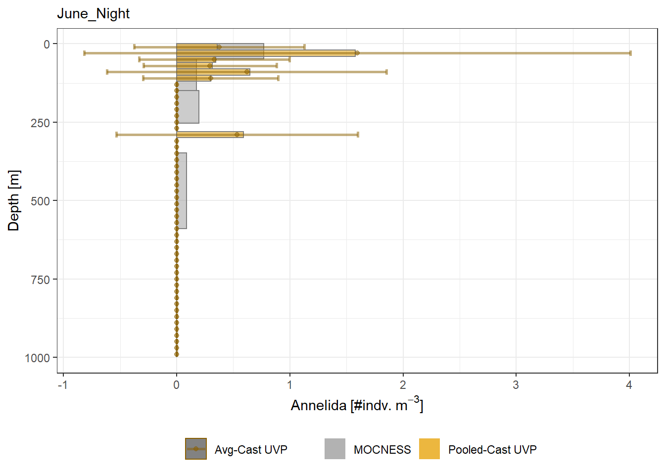
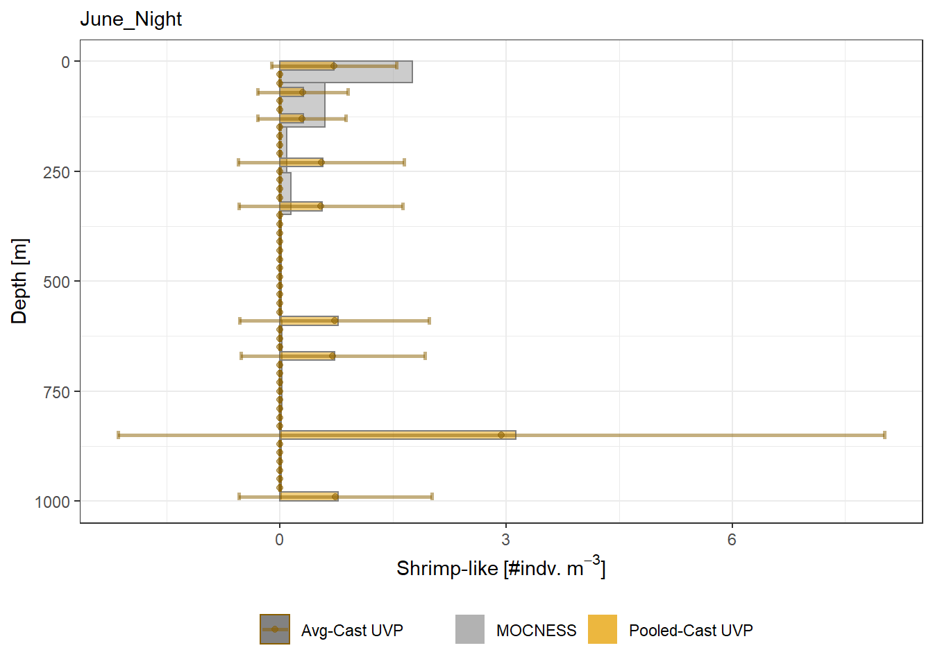
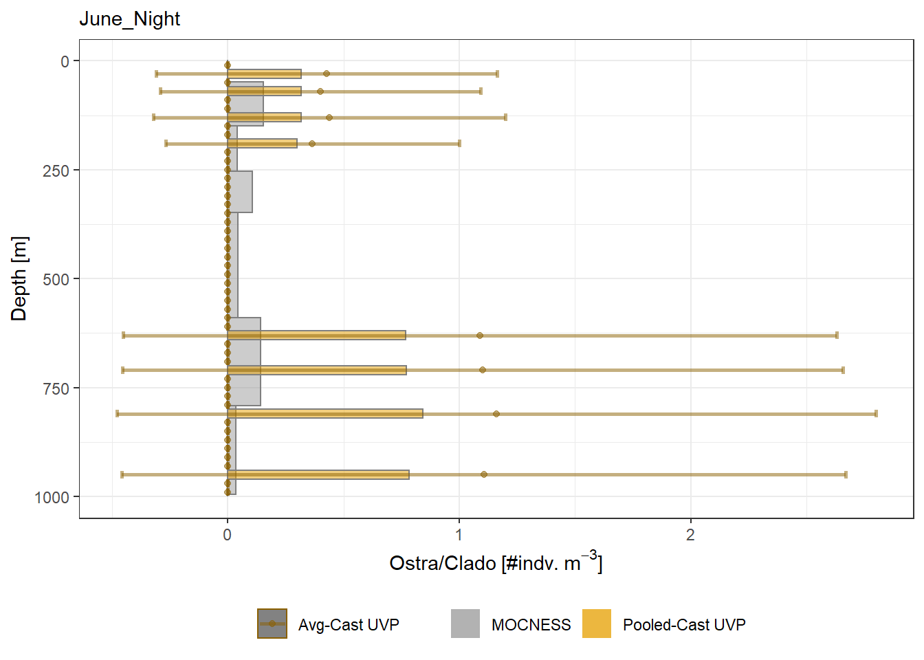
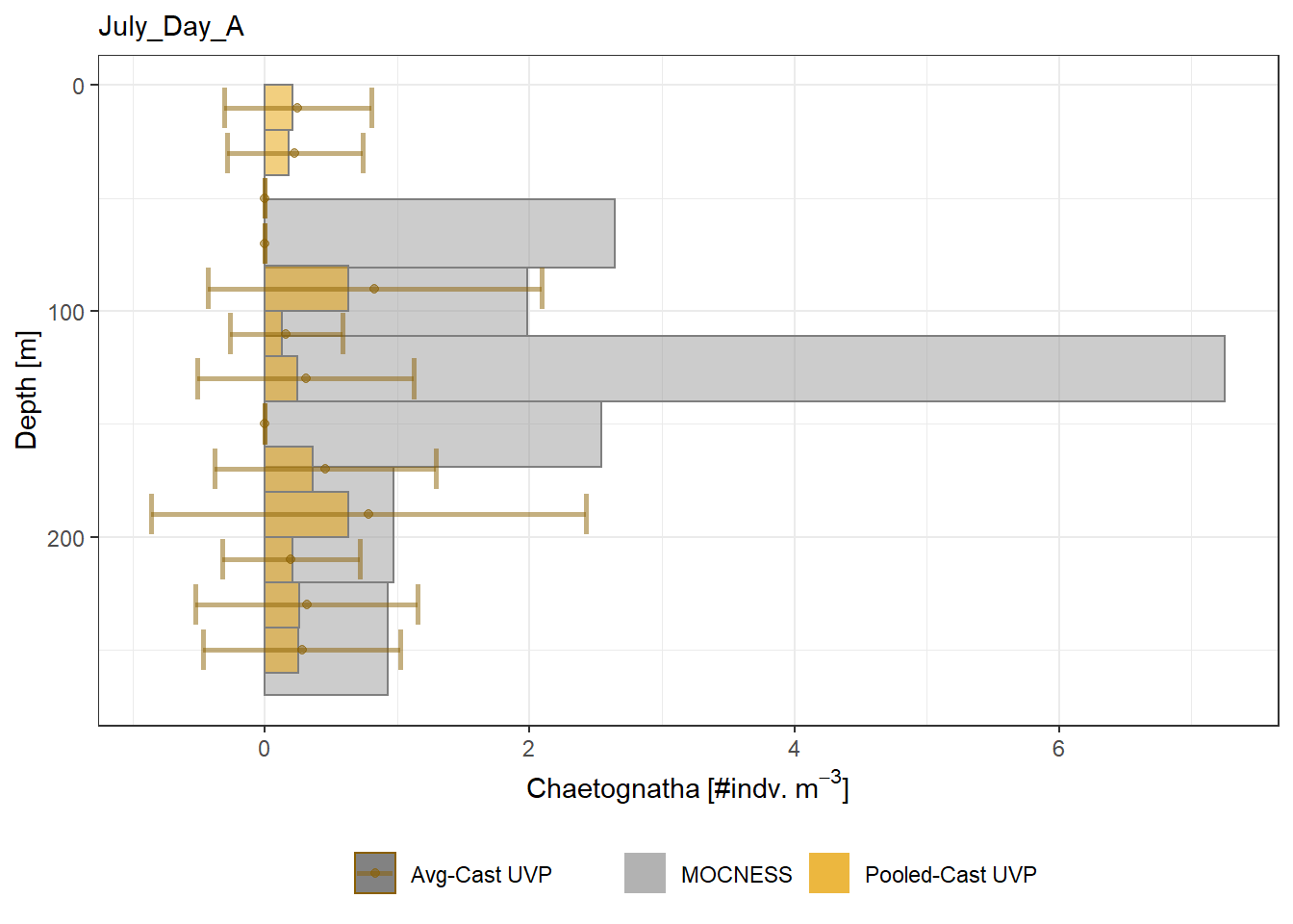
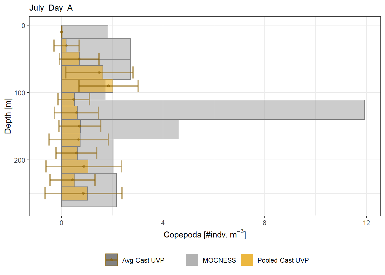
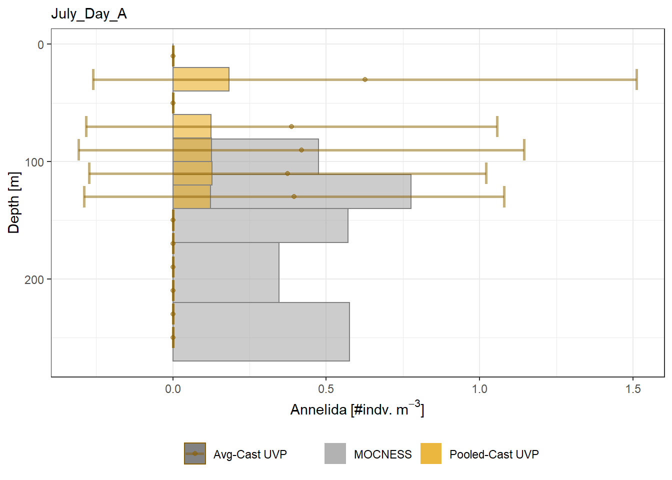
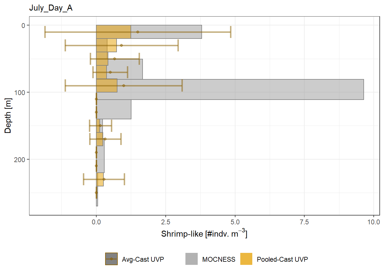
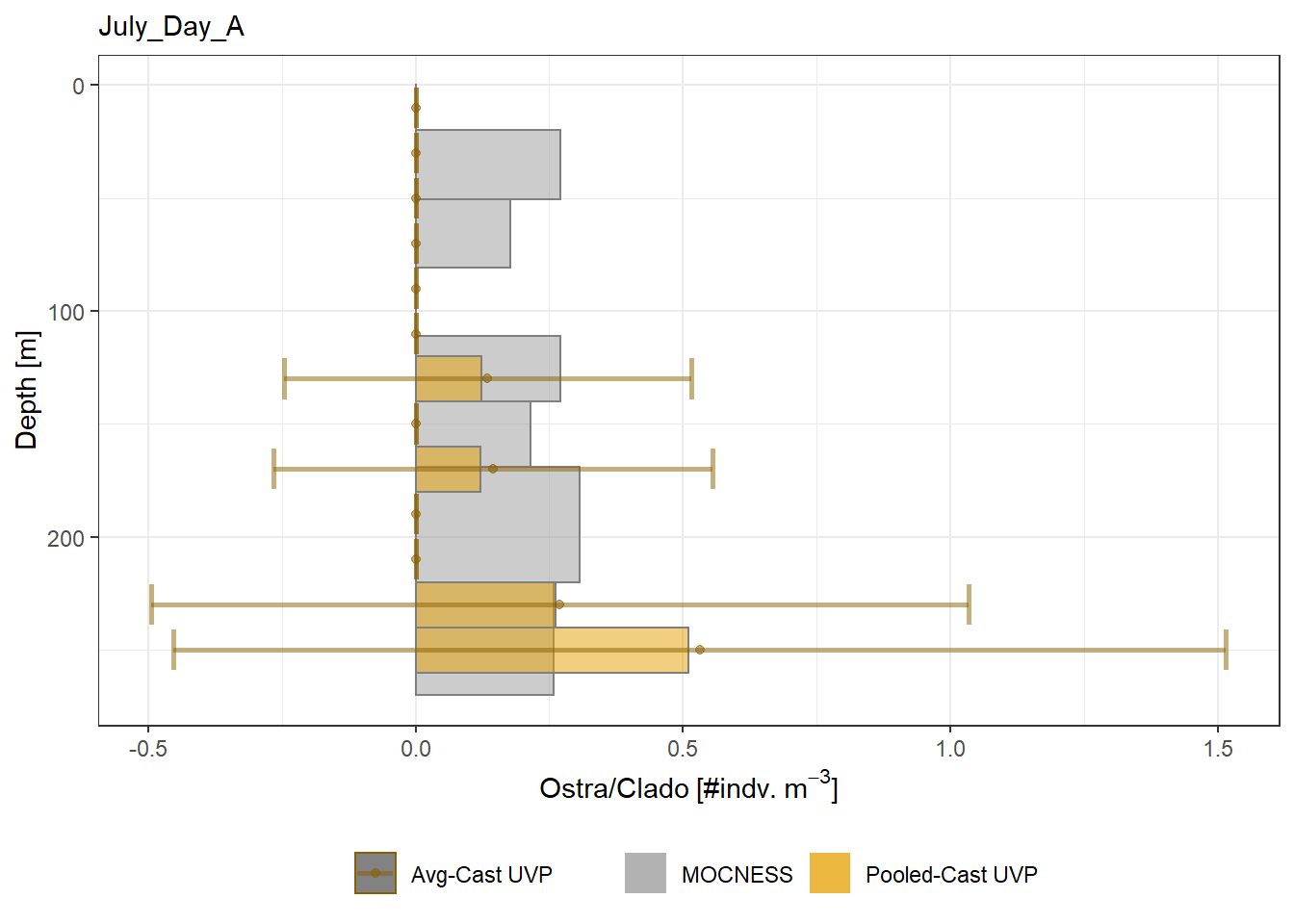
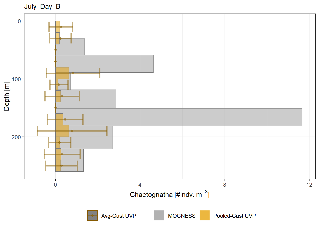
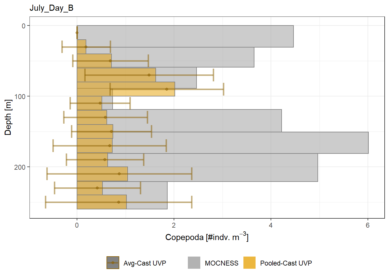
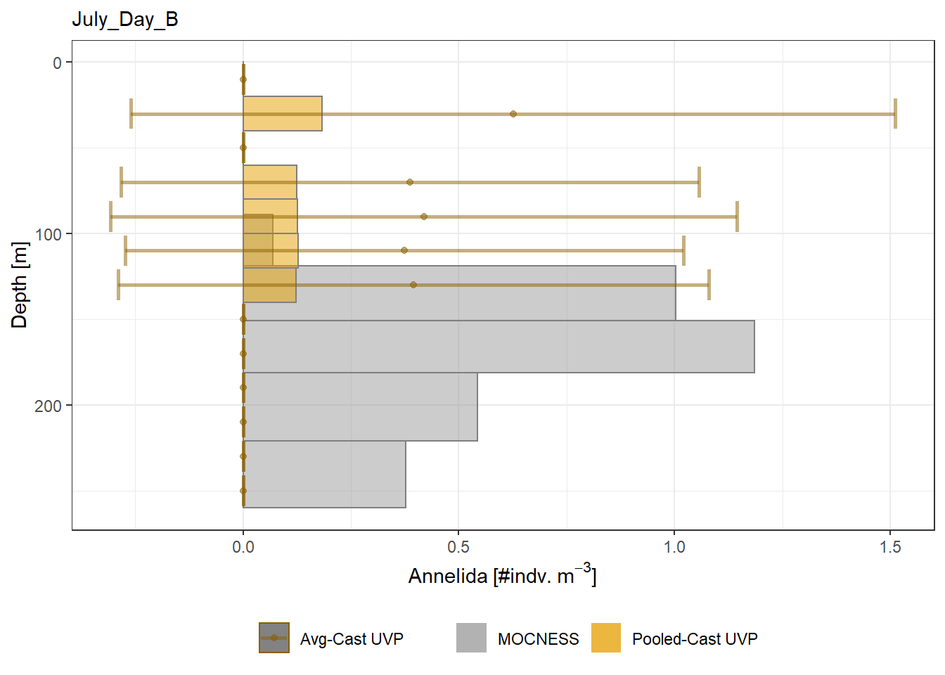
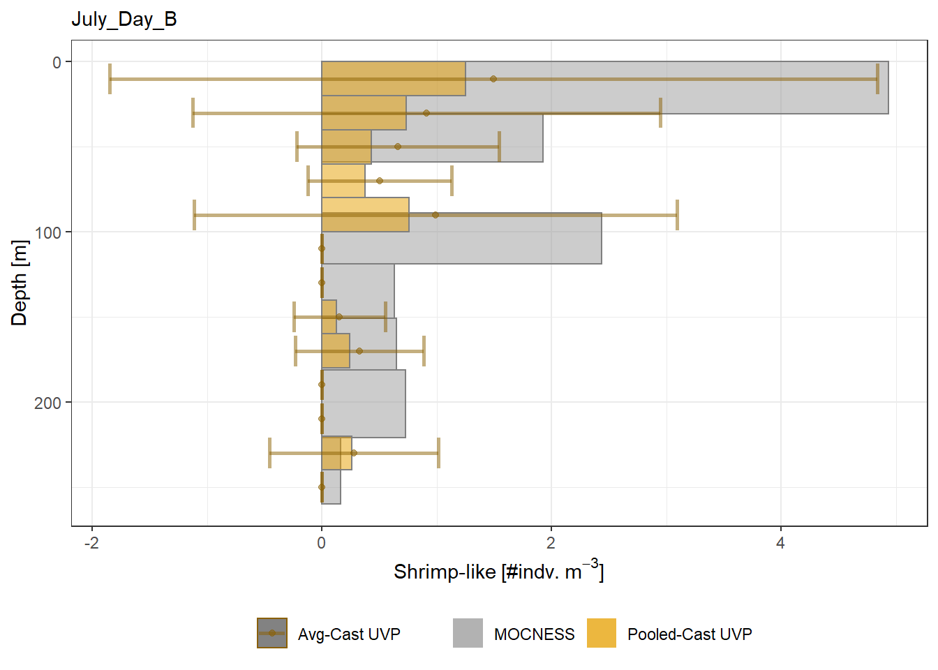
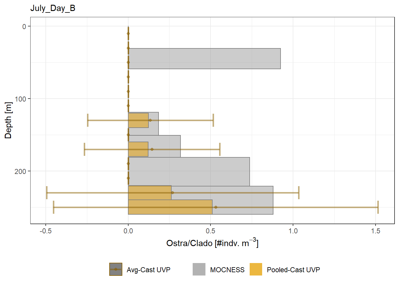
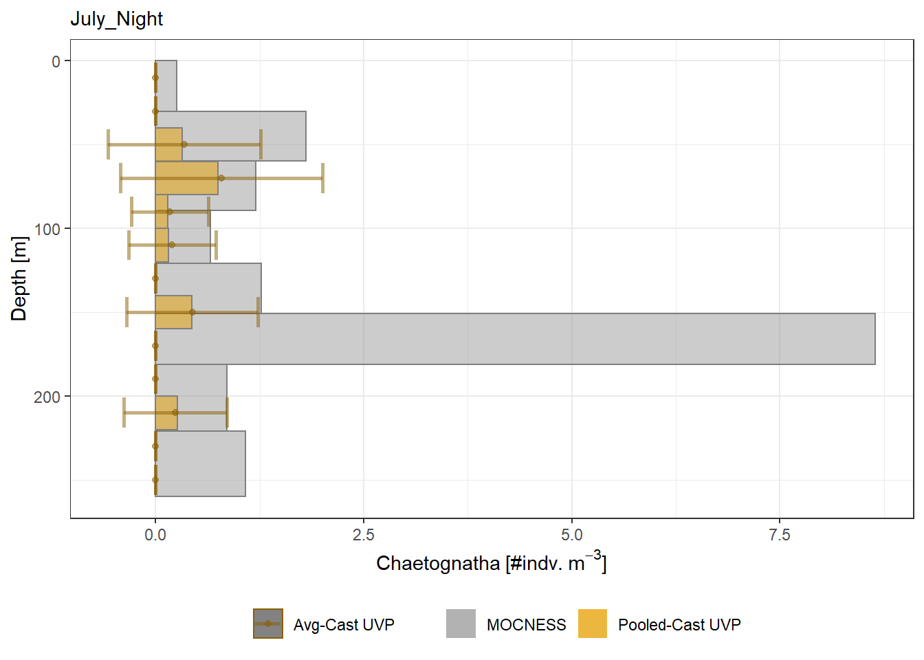
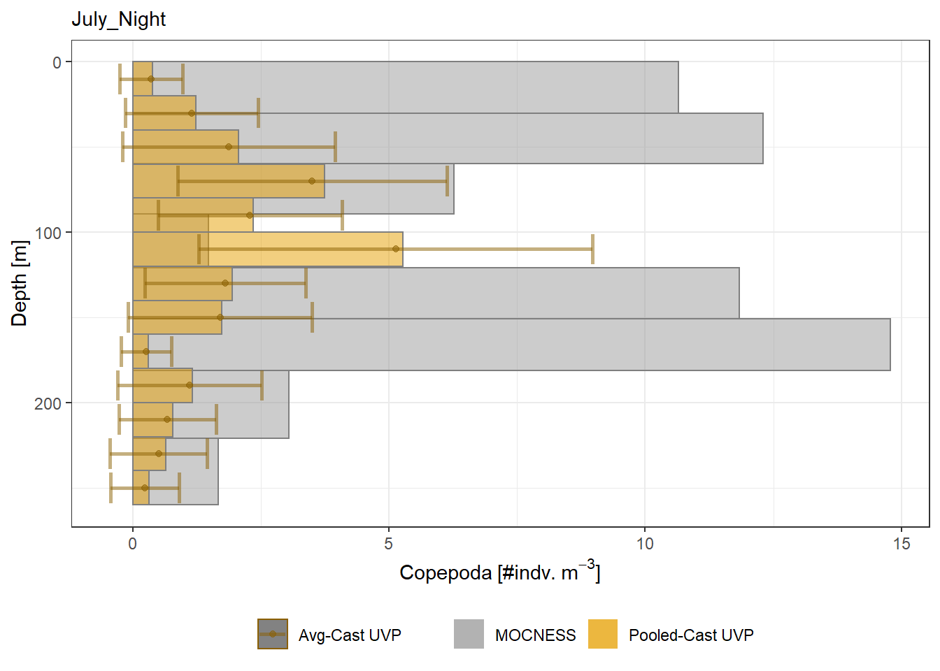
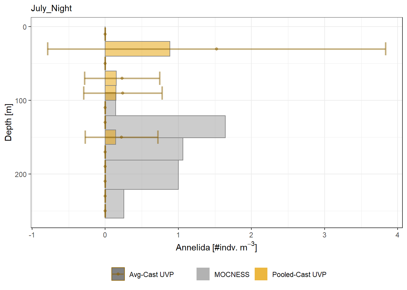
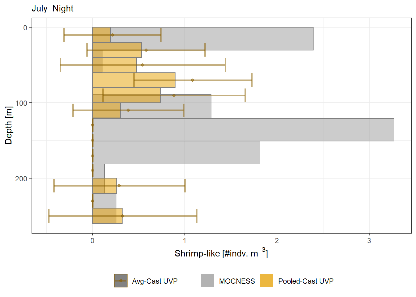
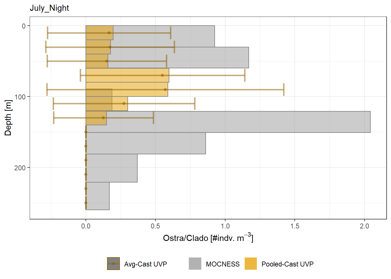
plot_list <- readRDS('../Output/main_fig_03_profile-density-comparison.rds')Density profiles of comparable taxa are shown when measured by the MOCNESS/ZOOSCAN and the UVP. UVP estimates were calculated two ways. In one method, similar UVP casts are pooled then the density of organisms in a depth bin were calculated \[\frac{\sum_{i}^{N}individuals_{i}}{\sum_{i}^{N}volume sampled_{i}}\]. The other method, density is calculated in individual uvp casts, then averaged between all similar casts: \[\frac{\sum_{i=1}^{N} \frac{individuals_{i}}{volume sampled_{i}}}{N}\] For all i casts, with a total of N casts.
rm(list = ls())
library(cowplot)
library(ggplot2)
plot_list <- readRDS('../Output/main_fig_03_profile-density-comparison.rds')plot_grid(for(i in 1:length(plot_list)){print(plot_list[[i]] + theme(legend.position = 'bottom'))}, ncol = 3)