Code
rm(list = ls())
library(ggplot2)

bw_plots <- readRDS('../Output/supp_fig_04_bin-width-integration.rds')The UVP records the exact depth position of each particle imaged. However, when estimating density, both in profiles or for depth-integration counts of plankton must be binned then concentration calculated. However bin width can impact these estimates. In this figure we investigated different bin-widths (between 1 - 100m) then determined how that impacted depth-integrated abundance estimates. Ideally the smallest bin-size should be used as this provides the most ecologically valuable information. However, too small of bins can impact depth-integration to be unstable estimates.
For this analysis, only casts which extended to, or beyond, 1000m were used. Depth integrated abundance was calculated for each casts for specific taxa then plotted:
rm(list = ls())
library(ggplot2)
bw_plots <- readRDS('../Output/supp_fig_04_bin-width-integration.rds')for(i in 1:length(bw_plots)){print(bw_plots[[i]]+theme(axis.text.x = element_text(size = 8)))}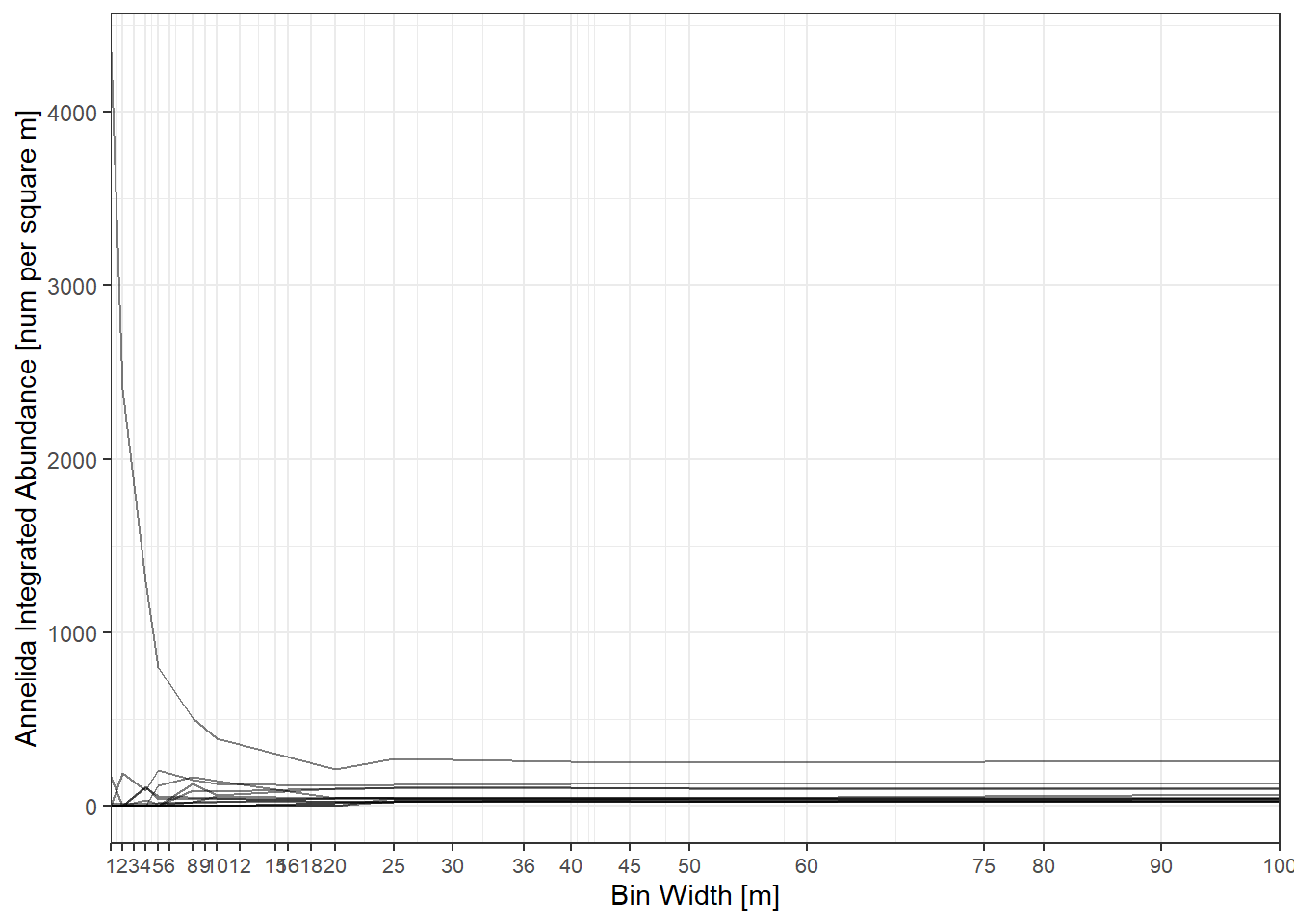
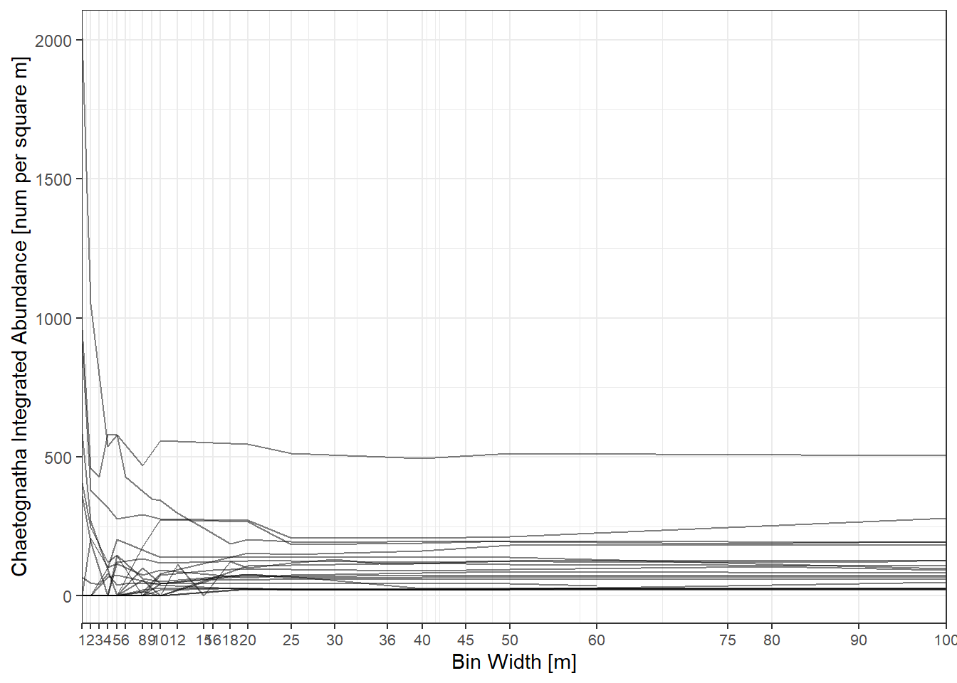
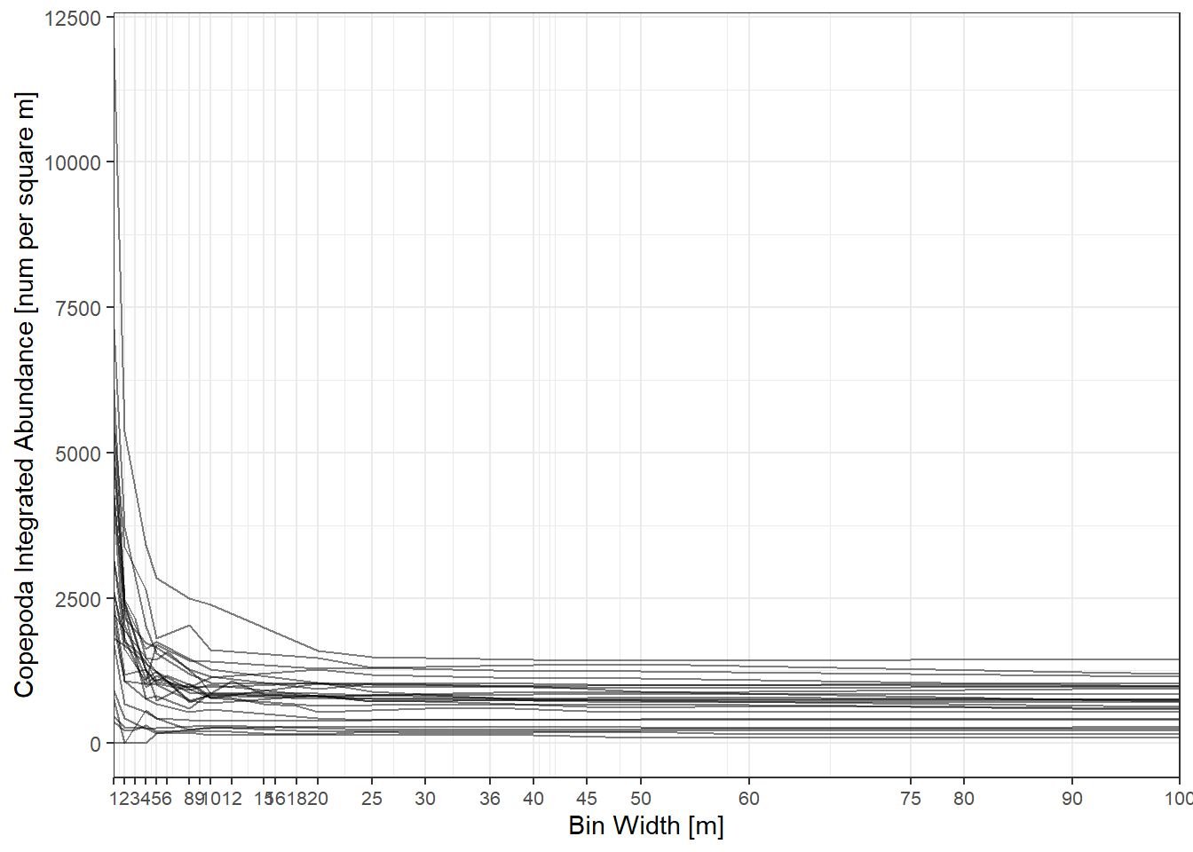
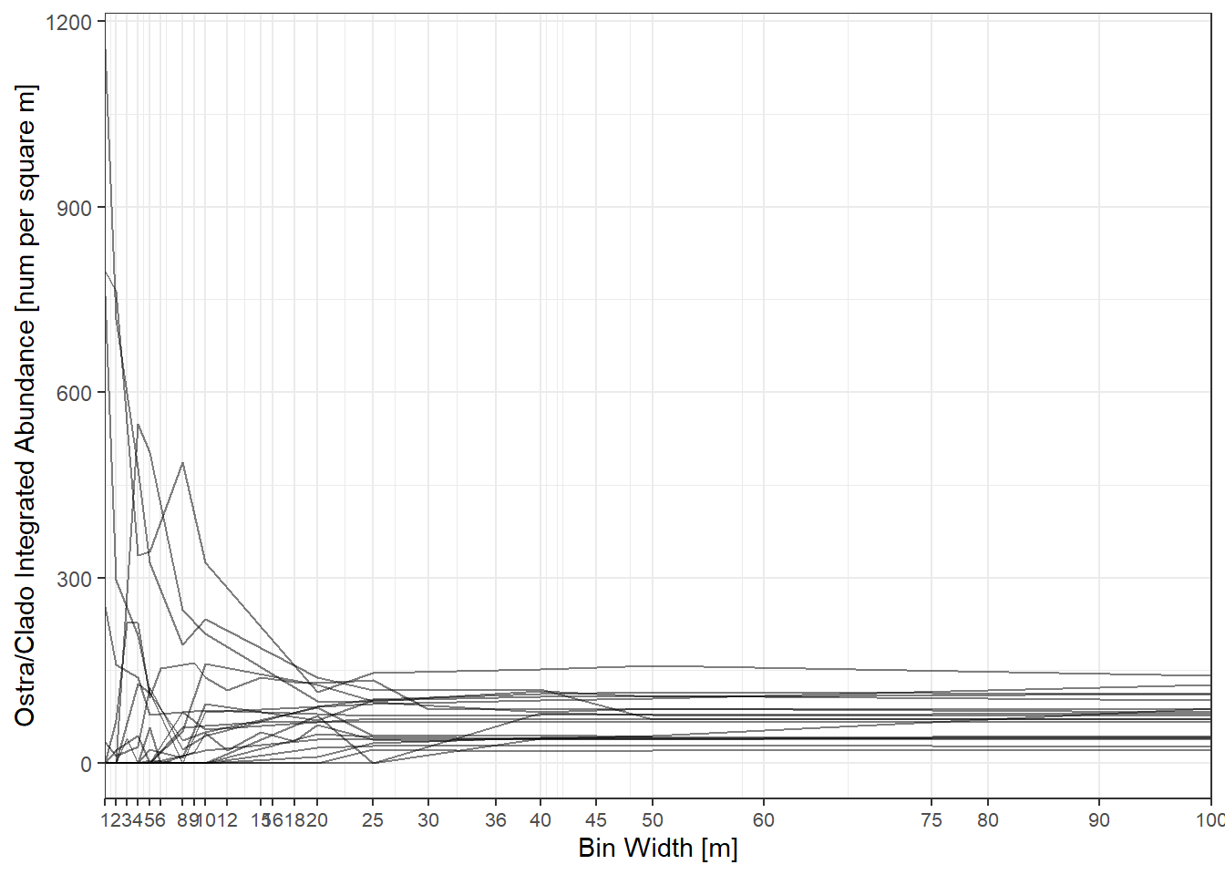
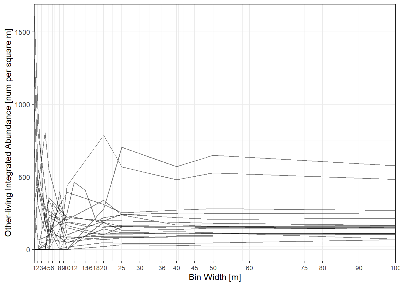
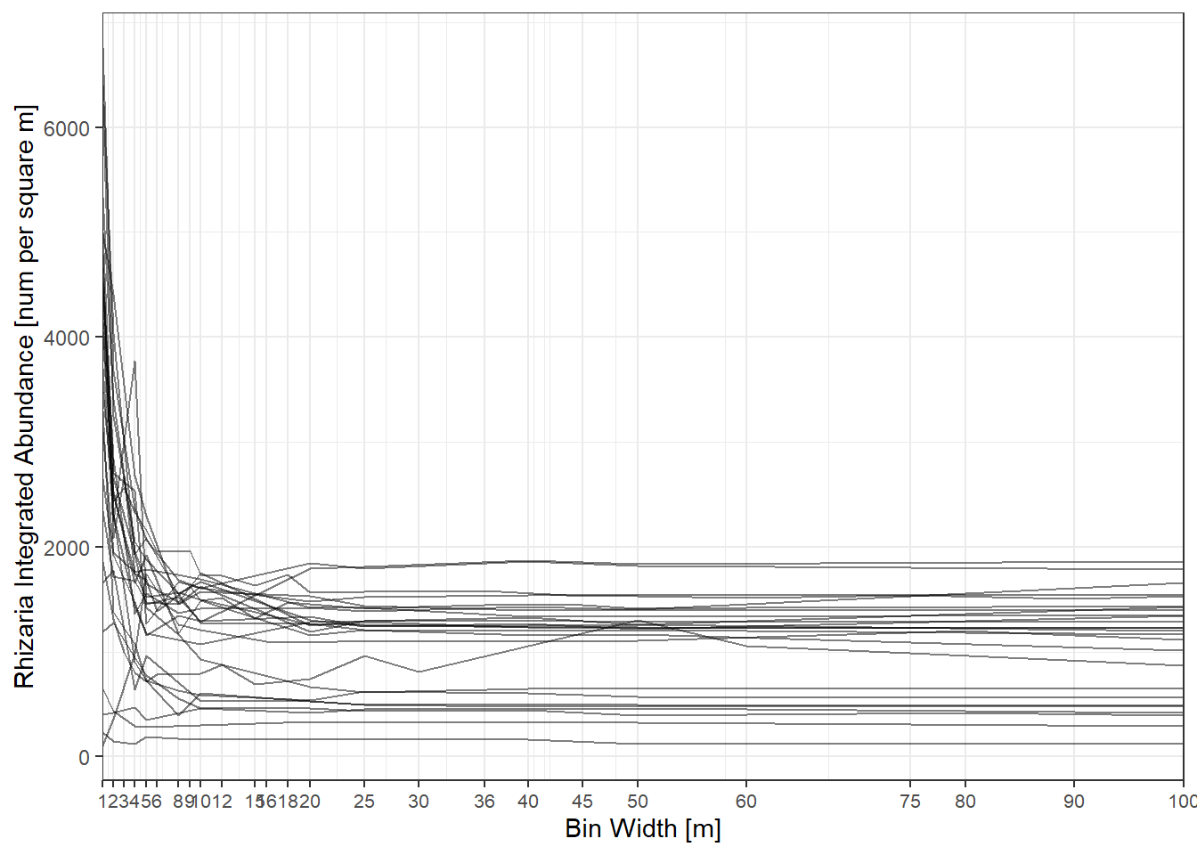

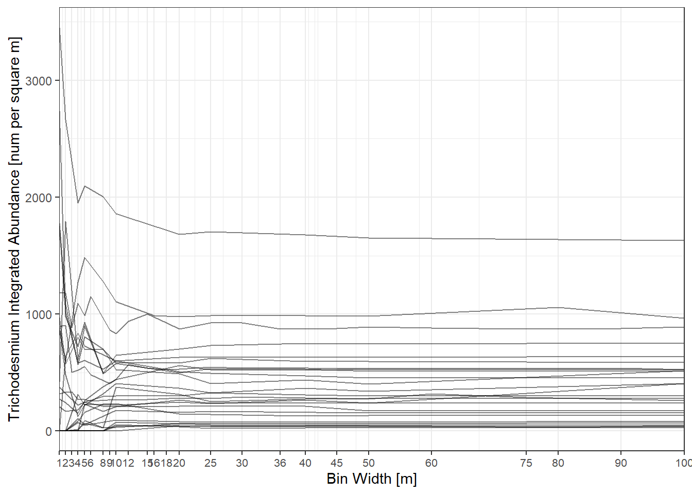

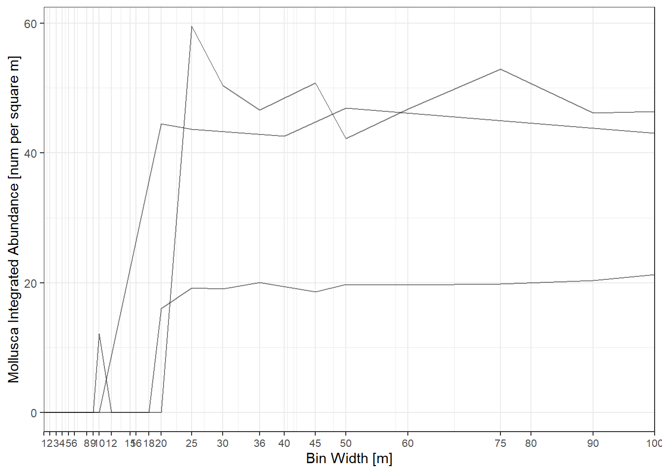
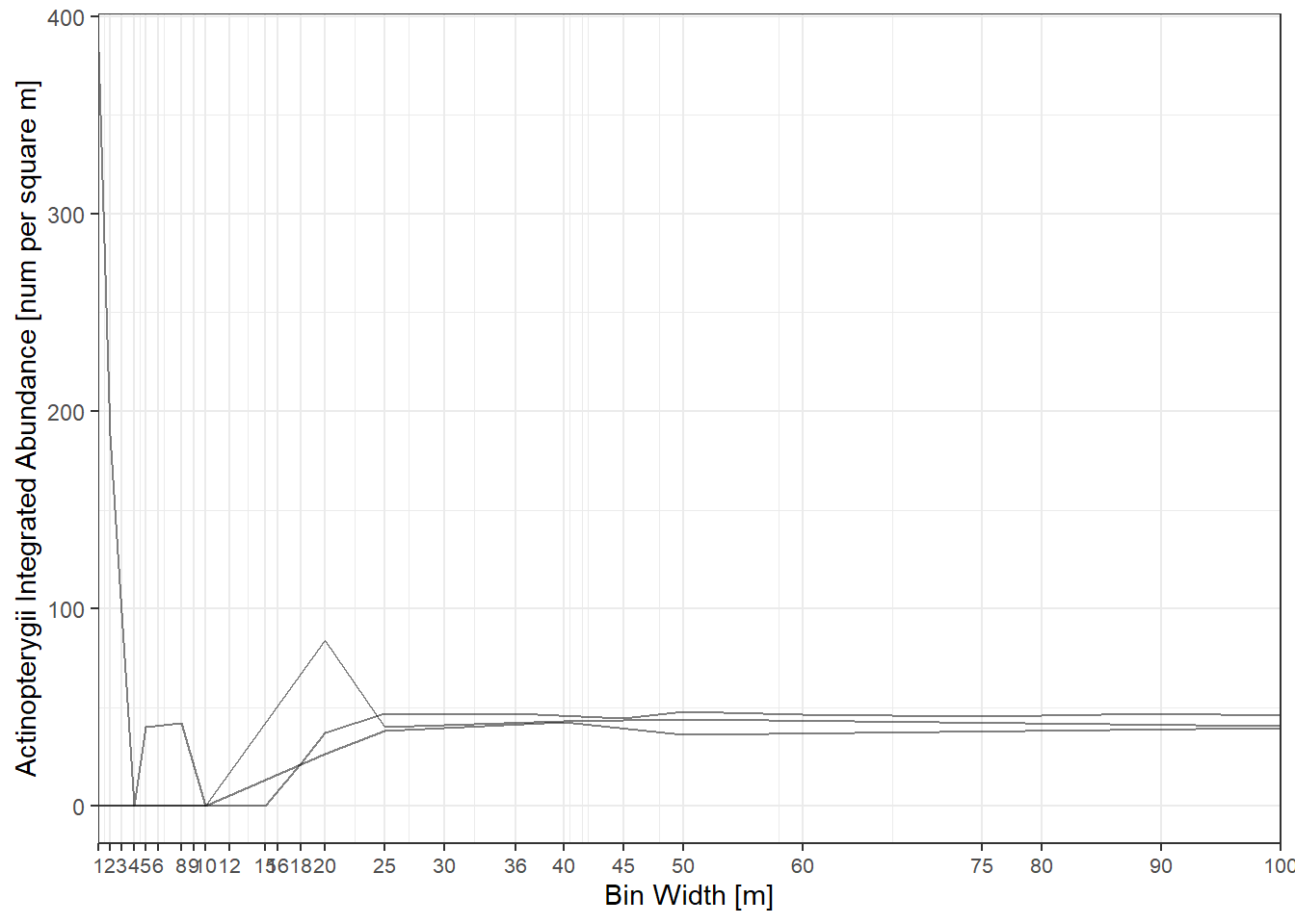
For some very sparse taxa (Mollusca, Actinopterygii) estimates are very unstable across bins and there were few casts which detected these organisms. However, for more abundant organisms, 20m appears to be a reliable bin-width.