Code
rm(list = ls())
library(ggplot2)
library(DT)

plot_list <- readRDS('../Output/supp_fig_01_full-size-distribution.rds')
dat_list <- readRDS('../Output/data_01_size-range-dfs.rds')As noted in the core paper, the MOCNESS samples a much larger range of sized-plankton than the UVP. For comparison, we look at MOCNESS-collected plankton which are equal to or larger than the smallest observed UVP plankton (0.934). The comparison of that size range can be found here. In this analysis, the full size range of the MOCNESS is shown. Additionally, the table below shows the proportion of MOCNESS-collected plankton which are excluded because they are smaller than 0.894mm
rm(list = ls())
library(ggplot2)
library(DT)
plot_list <- readRDS('../Output/supp_fig_01_full-size-distribution.rds')
dat_list <- readRDS('../Output/data_01_size-range-dfs.rds')print(plot_list)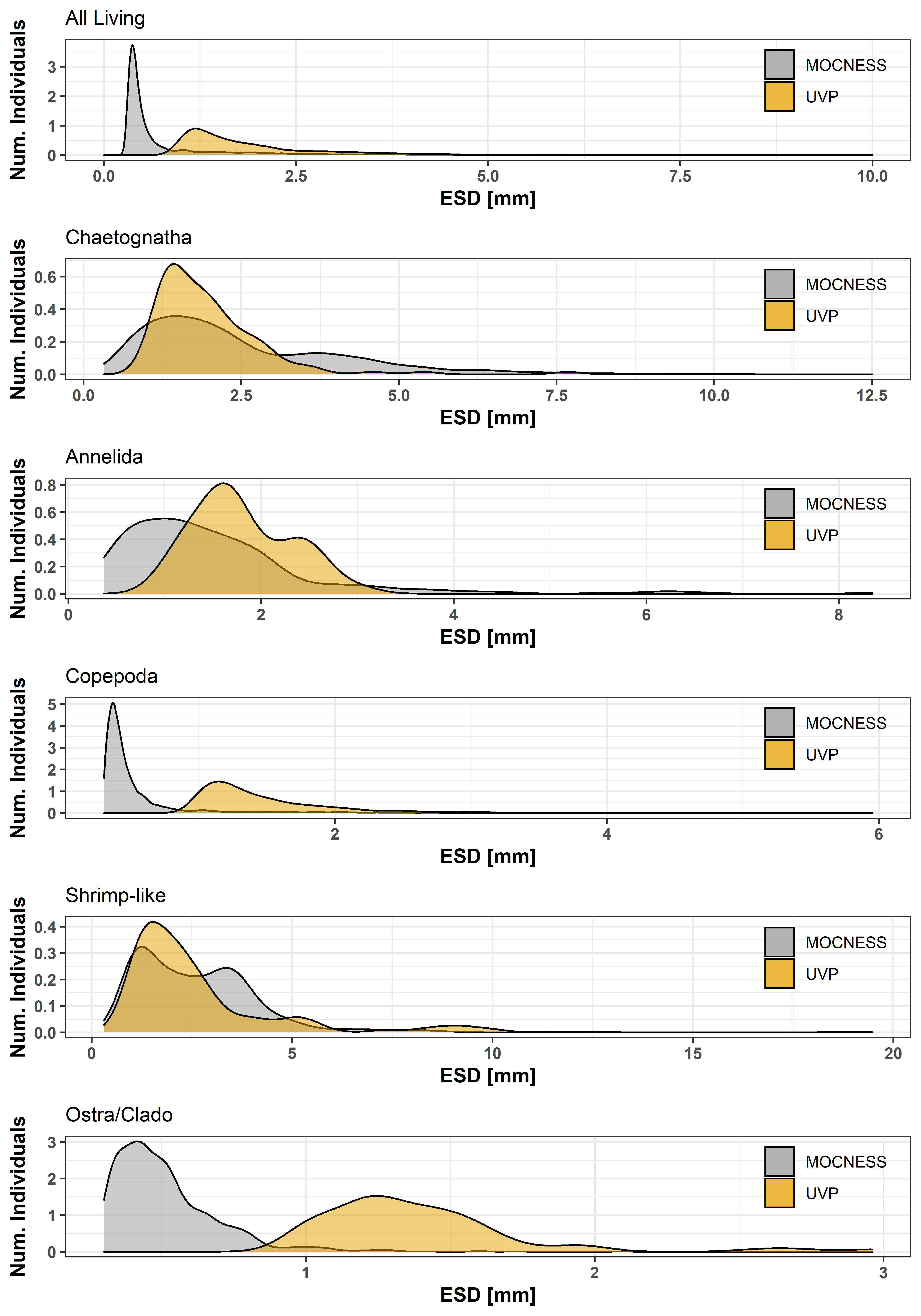
comp_taxo <- c('Chaetognatha', 'Annelida', 'Copepoda', 'Shrimp-like',
               'Ostra/Clado')

moc_dat <- dat_list$moc_full
moc_dat <- moc_dat[moc_dat$taxo_name %in% comp_taxo,]

get_percentile <- function(taxo) {
  value <- ecdf(moc_dat$calc_esd[moc_dat$taxo_name == taxo])(0.934)
  return(round(value*100, 2))
}

moc_tab <- data.frame(
  taxa = sort(unique(moc_dat$taxo_name)),
  `% Moc Excluded` = sapply(sort(unique(moc_dat$taxo_name)),
                            get_percentile)
)

datatable(moc_tab, class = 'hover', colnames = c('Taxa', '% Moc Excluded'),
          rownames = FALSE, caption = 'Mocness-collected taxa and percent excluded by 0.894 size cut off')