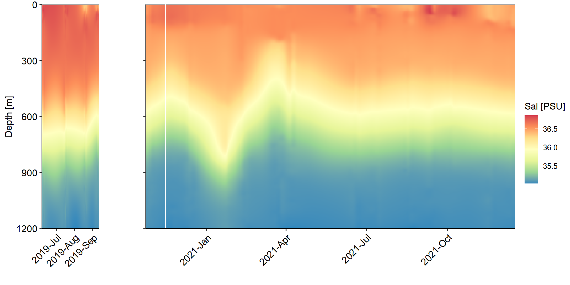
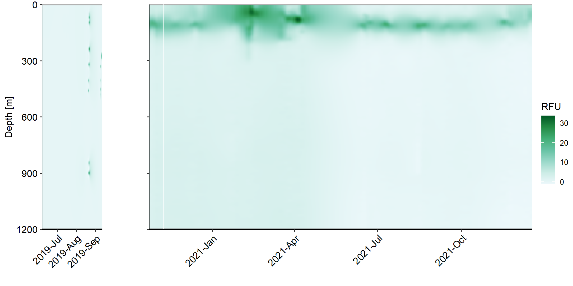
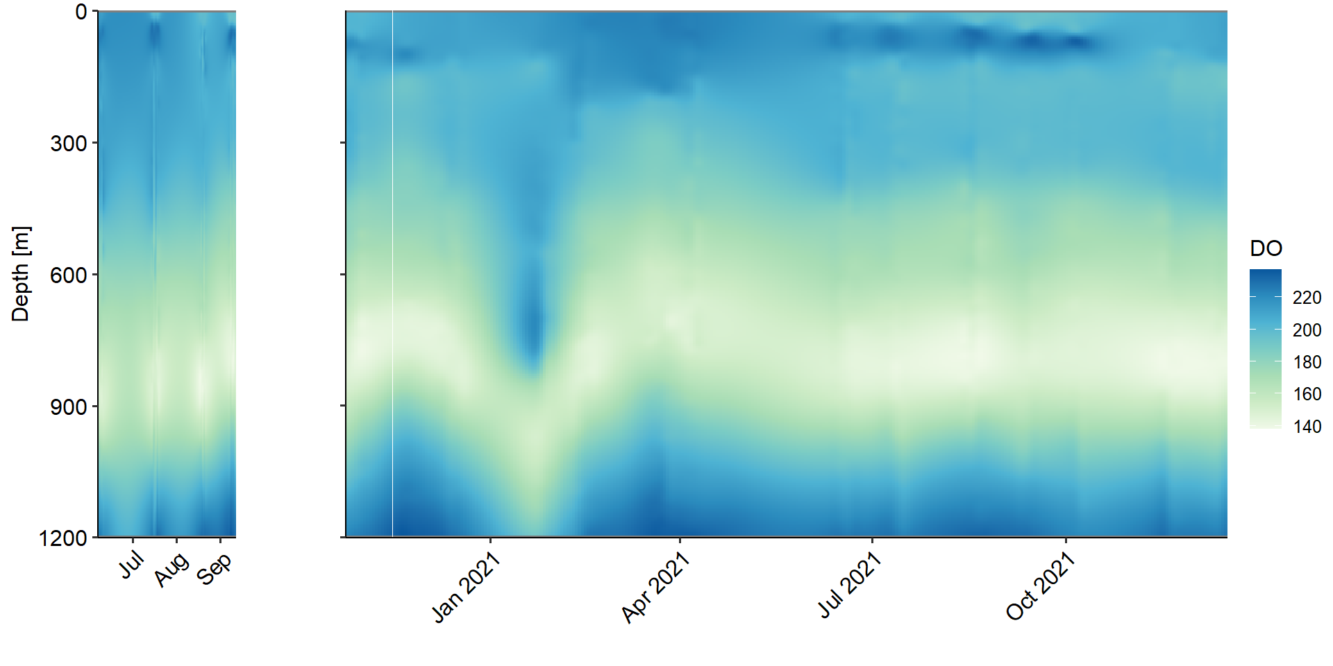
Physical Backdrop - water column parameters across study period

Over the course of the cruises, there was some seasonal variation. Figures below show the change in Salinity, Temperature, Chlorophyll, and Dissolved Oxygen

Code

rm(list = ls())
library(ggplot2)
library(ggpubr)
full_proj_values <- readRDS('../data/ctd_02_interp-grid.rds')$full_proj

ODV_colours <- c("#feb483", "#d31f2a", "#ffc000", "#27ab19", "#0db5e6", "#7139fe", "#d16cfa")

# set up
value_class <- function(cruise){
  ret_list <- vector('list',4)
  names(ret_list) <- c('Sal',"Temperature",'RFU','DO')
  return(ret_list)
}

full_proj_plot <- list()
full_proj_plot$early <- value_class()
full_proj_plot$late <- value_class()


# |- Plotting -----------------------
for(i in 1:length(full_proj_plot)) {
  
  full_proj_plot[[i]]$Sal <- ggplot()+
    geom_tile(data = full_proj_values[[i]]$Sal,
              aes(x = Date,
                  y = Depth,
                  fill = Sal)) +
    scale_y_reverse()+
    scale_fill_distiller(palette = 'Spectral')+
    scale_color_manual(breaks = c('day','night'),
                       values = c('grey','black'))+
    scale_x_datetime(date_labels = '%Y-%b')+
    labs(x = "",y = "Depth [m]", fill = "Sal [PSU]",
         color = "")+
    theme_pubr()+
    theme(legend.position = 'right')+
    coord_cartesian(expand = 0)
  
  full_proj_plot[[i]]$Temperature <- ggplot()+
    geom_tile(data = full_proj_values[[i]]$Temperature,
              aes(x = Date,
                  y = Depth,
                  fill = Temperature)) +
    scale_y_reverse()+
    scale_x_datetime(date_labels = '%Y-%b')+
    scale_fill_gradientn(colors = rev(ODV_colours))+
    scale_color_manual(breaks = c('day','night'),
                       values = c('grey','black'))+
    labs(x = "",y = "Depth [m]", fill = "Temperature",
         color = "")+
    theme_pubr()+
    theme(legend.position = 'right')+
    coord_cartesian(expand = 0)
  
  full_proj_plot[[i]]$RFU <- ggplot() + 
    geom_tile(data = full_proj_values[[i]]$RFU,
              aes(x = Date,
                  y = Depth,
                  fill = RFU)) +
    scale_y_reverse()+
    scale_x_datetime(date_labels = '%Y-%b')+
    scale_fill_distiller(palette = 'BuGn',
                         direction = 1)+
    scale_color_manual(breaks = c('day','night'),
                       values = c('grey','black'))+
    labs(x = "",y = "Depth [m]", fill = "RFU",
         color = "")+
    theme_pubr()+
    theme(legend.position = 'right')+
    coord_cartesian(expand = 0)
  
  full_proj_plot[[i]]$DO <- ggplot() + 
    geom_tile(data = full_proj_values[[i]]$DO,
              aes(x = Date,
                  y = Depth,
                  fill = DO)) +
    scale_y_reverse()+
    scale_fill_distiller(palette = 'GnBu',
                         direction = 1)+
    scale_color_manual(breaks = c('day','night'),
                       values = c('grey','black'))+
    labs(x = "",y = "Depth [m]", fill = "DO",
         color = "")+
    theme_pubr()+
    theme(legend.position = 'right')+
    coord_cartesian(expand = 0)
  
}

Code

ggarrange(full_proj_plot$early$Sal +
            theme(axis.text.x = element_text(angle = 45,
                                             hjust = 1,
                                             vjust = 1)),
          full_proj_plot$late$Sal +
            theme(axis.text.y = element_blank(),
                  axis.text.x = element_text(angle = 45,
                                             hjust = 1,
                                             vjust = 1))+
            labs(y = ""),
          common.legend = T,
          legend = 'right',
          nrow = 1,
          widths = c(0.2,0.8),
          align = 'hv')

Figure 1a. Salinity values across whole study period interpolated from ctd casts.

Code

ggarrange(full_proj_plot$early$Temperature +
            theme(axis.text.x = element_text(angle = 45,
                                             hjust = 1,
                                             vjust = 1)),
          full_proj_plot$late$Temperature +
            theme(axis.text.y = element_blank(),
                  axis.text.x = element_text(angle = 45,
                                             hjust = 1,
                                             vjust = 1))+
            labs(y = ""),
          common.legend = T,
          legend = 'right',
          nrow = 1,
          widths = c(0.2,0.8),
          align = 'hv')

Figure 1b. Temperature values across whole study period interpolated from ctd casts.

Code

ggarrange(full_proj_plot$early$RFU +
            theme(axis.text.x = element_text(angle = 45,
                                             hjust = 1,
                                             vjust = 1)),
          full_proj_plot$late$RFU +
            theme(axis.text.y = element_blank(),
                  axis.text.x = element_text(angle = 45,
                                             hjust = 1,
                                             vjust = 1))+
            labs(y = ""),
          common.legend = T,
          legend = 'right',
          nrow = 1,
          widths = c(0.2,0.8),
          align = 'hv')

Figure 1c. RFU values across whole study period interpolated from ctd casts.

Code

ggarrange(full_proj_plot$early$DO +
            theme(axis.text.x = element_text(angle = 45,
                                             hjust = 1,
                                             vjust = 1)),
          full_proj_plot$late$DO +
            theme(axis.text.y = element_blank(),
                  axis.text.x = element_text(angle = 45,
                                             hjust = 1,
                                             vjust = 1))+
            labs(y = ""),
          common.legend = T,
          legend = 'right',
          nrow = 1,
          widths = c(0.2,0.8),
          align = 'hv')

Figure 1d. DO values across whole study period interpolated from ctd casts.